Modelling of two phase flow in packed bed (continued)

[Chestermiller]

Those changes had been incorporated anyway. The plots above (post #268) are the plots you mentioned earlier and use as much of the Tuinier data as possible. In places I had to make assumptions (like picking very high $U_g$ and $U_b$ values to approximate their infinite gas-solid heat transfer coefficient). Unless I've read the plots incorrectly they're not very similar yet. I'm looking into the possibility that I've forgotten to convert between kg and mol somewhere along the way

Those new graphs in #268 are encouraging to me. Some questions:

1. Why didn't you show temperatures from -90 to 100 C?

2. Although they use infinite U's and we use finite U's, our U's are still pretty high, as evidenced by the very small differences between the gas temperature and the bed temperature. What do our results look like using our correlations.

3. There seems to be a time scaling issue here. Are you sure you are showing the results at the correct times? Are you using fixed time interval, or having the integrator spit out results at specified times? The time scaling factor seems to be something like 10x.

Maybe I've misunderstood again but this plot (Fig 7 in Tuinier) doesn't seem to make sense):
View attachment 304867
The x-axis is time in seconds and the temperature is the outlet temperature of the packed bed. Does this not say that their temperature reaches a maximum at roughly -90C also? But surely this is at odds with Fig 6 and 5 which show the temperature going above this. Or have I misunderstood? Because fig 7 looks a lot like our time vs Tg plot (besides the time scale)

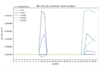
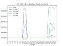
It looks like the operating conditions for Fig.7 were a little different than for figs. 5 & 6. I wouldn't worry too much about this.

 

[casualguitar]

1. Why didn't you show temperatures from -90 to 100 C?

Because the temperature only rises to about -90C for some reason. I can run the simulation for much longer times but the temperature will max out at -90C

Although they use infinite U's and we use finite U's, our U's are still pretty high, as evidenced by the very small differences between the gas temperature and the bed temperature. What do our results look like using our correlations.

I haven't added in these correlations yet given the above issue. I think we agreed earlier its better to fix that first rather than add the U correlations in and then fix. But if necessary I can add these

3. There seems to be a time scaling issue here. Are you sure you are showing the results at the correct times? Are you using fixed time interval, or having the integrator spit out results at specified times? The time scaling factor seems to be something like 10x.

I think so anyway. So I pass t_eval to the integrator with is an array of times that I would like the solution stored at. I just store the time at each second interval. I also checked the length of the time array output by the integrator and it is the same length as the simulation time, surely indicating that there is no time scaling issue?

 

[Chestermiller]

Because the temperature only rises to about -90C for some reason. I can run the simulation for much longer times but the temperature will max out at -90C

How can they not get higher than -90 C at short distances from the inlet? The stream coming in is at 100 C.

I haven't added in these correlations yet given the above issue. I think we agreed earlier its better to fix that first rather than add the U correlations in and then fix. But if necessary I can add these

Yes, please turn them on and see what we get.

I think so anyway. So I pass t_eval to the integrator with is an array of times that I would like the solution stored at. I just store the time at each second interval. I also checked the length of the time array output by the integrator and it is the same length as the simulation time, surely indicating that there is no time scaling issue?
View attachment 304868

We seem to be losing a factor of 10 elsewhere then. It's hard to imagine where, unless it is the individual tank holdup time (molar holdup divided by molar flow rate).

 

[casualguitar]

How can they not get higher than -90 C at short distances from the inlet? The stream coming in is at 100 C.

Exactly. However I mentioned yesterday if we scale down the heats of vaporisation/sublimation the temperature does go above -90C and reaches 100C. Obviously we can't just change those values though. But in effect by scaling these down we're actually scaling down $Q_{GI}$ and $Q_{IB}$ because these are a function of the heats of vaporisation/sublimation. I'm not sure why scaling down these values let's the temperature increase up to the inlet temperature but it does for some reason. As you say we're missing a factor of 10 somewhere (or possibly a factor greater than 10)

Yes, please turn them on and see what we get.

Will do. This will take a bit of time

We seem to be losing a factor of 10 elsewhere then. It's hard to imagine where, unless it is the individual tank holdup time (molar holdup divided by molar flow rate).

I agree there is a factor of 10 (or greater) lost somewhere, I'll add those $U_g$ values in anyway and see what happens

 

[casualguitar]

I found one potential factor of 10 loss relating to the inlet molar flow

The Tuinier et al paper uses 0.27 kg/m2.s. I converted this to mol/m2.s (x1000/mW)

Now to convert to molar flow I was multiplying by $A_C$, but is this correct? Or should I be multiplying by the actual flow area which I think would be A_c * epsilon? Including a voidage term min the inlet flow rate term makes a difference in how 'spread out' the variation is.

It doesn't help the temperature reach the inlet temperature unfortunately though but its a start

 

[Chestermiller]

No. This is always given based on the column area Ac.

 

[Chestermiller]

What do you get for the molar flow rate? Assuming a uniform temperature of 300K and a pressure of 1 atm, what do you get for the gas holdup in moles?

 

[casualguitar]

What do you get for the molar flow rate? Assuming a uniform temperature of 300K and a pressure of 1 atm, what do you get for the gas holdup in moles?

I was about to comment in relation to this. Printing the reynolds numbers at each position results in values around Re = 100, which are possibly quite low

For a molar flux of 0.27kg/m2.s as used in Tuinier et al, I get a molar flow of 0.0085mol/s, which gives a gas holdup of 0.0012 mol at a temperature of 300K and 1 atm. Does this seem reasonable?

Also I've implemented the variable $U_g$ values. They do change the plots slightly (not too much). Also printing out these $U_g$ values gives values in the range of about 20 to 60 W/m2.K

Here are the plots for non-constant $U_g$:

Edit: I missed the molar flow rate question.

So the inlet flow is 0.0085mol/s. In the first tank this actually increases up to 0.01 mol/s and stays at about this value throughout the simulation. In the other tanks it also does an initial jump up to 0.01mol/s but then gradually tails off down to about 0.005 mol/s which is more what I would have expected, indicating I've possibly set this up incorrectly at the boundary

 

[Chestermiller]

I was about to comment in relation to this. Printing the reynolds numbers at each position results in values around Re = 100, which are possibly quite low

For a molar flux of 0.27kg/m2.s as used in Tuinier et al, I get a molar flow of 0.0085mol/s, which gives a gas holdup of 0.0012 mol at a temperature of 300K and 1 atm. Does this seem reasonable?

The molar flow rate seems reasonable, but not the holdup. I get a superficial column volume of 289 cc, and, assuming a void fraction of 0.32, I get a column void volume of 92.4 cc = 0.0924 liters. From the ideal gas law at 1 atm and 300 K, I get a molar density of 0.041 moles/liter. So, for a molar holdup, I get 0.0038 moles. So for a mean residence time of the gas, I get 0.0038/.0085 = 0.45 seconds. This is way less than the times we are seeing in our calculations for a temperature wave to travel through the bed, so the solid bed must be having a substantial effect of the speed of temperature waves through the column. Apparently, in our model, the waves are slowed much more than in the Turnier model.

 

[casualguitar]

This is way less than the times we are seeing in our calculations for a temperature wave to travel through the bed, so the solid bed must be having a substantial effect of the speed of temperature waves through the column. Apparently, in our model, the waves are slowed much more than in the Turnier model.

I've calculated the molar holdup by saying that:

$$m_j = \frac{P}{RT_g}A_C*\delta z*\epsilon$$

This is way less than the times we are seeing in our calculations for a temperature wave to travel through the bed,

If these times were increased, is it correct to say that we would see the temperature variation 'spread out' across the bed rather than be concentrated at the inlet?

 

[casualguitar]

The molar flow rate seems reasonable, but not the holdup

If the molar flow is ok, and the molar holdup is dependent on the molar flow, surely this means the bug is in the molar holdup equation itself (rather than in any question that feeds the molar holdup equation)?

 

[Chestermiller]

I've calculated the molar holdup by saying that:

$$m_j = \frac{P}{RT_g}A_C*\delta z*\epsilon$$

If these times were increased, is it correct to say that we would see the temperature variation 'spread out' across the bed rather than be concentrated at the inlet?

The value I calculated was for the entire column, not 1 tank. Our values should differ by a factor of 30. Your value was 0.0012 for a single tank, and mine would be 0.00012 moles for a single tank, a factor of 10 lower. I've checked my number, and it seems correct. please check yours.

 

[Chestermiller]

If the molar flow is ok, and the molar holdup is dependent on the molar flow, surely this means the bug is in the molar holdup equation itself (rather than in any question that feeds the molar holdup equation)?

Your molar holdup equation looks correct.

 

[casualguitar]

The value I calculated was for the entire column, not 1 tank. Our values should differ by a factor of 30. Your value was 0.0012 for a single tank, and mine would be 0.00012 moles for a single tank, a factor of 10 lower. I've checked my number, and it seems correct. please check yours.

Heres the exact molar holdup calculation:

And here's the output:

Other values:
Bed length = 3m
Bed diameter = 0.035m
n = 30
dz = bed length/n

Possibly the most likely different value is the bed diameter. Are you also using 0.035m?

 

[Chestermiller]

Heres the exact molar holdup calculation:
View attachment 304982
And here's the output:
View attachment 304983

Other values:
Bed length = 3m
Bed diameter = 0.035m
n = 30
dz = bed length/n

Possibly the most likely different value is the bed diameter. Are you also using 0.035m?

Their bed length is 0.3 m, not 3m.

 

[casualguitar]

Their bed length is 0.3 m, not 3m.

Whoops my mistake. I changed that and now yes I'm getting 0.00012 moles also for a single tank

Here are the plots with the correct bed length:

What I noticed was that this 'max levelling off temperature' of around -85C is not constant. If I zoom in:

The temperature at the inlet seems to actually slightly decrease over time

These plots are definitely quite a bit closer to the Tuinier plots though. The main things that are not the same are the temperature profiles near the inlet (not sure why the temperature doesn't increase further than -86C, and also possible the max mass deposition in our simulation being about double what is seen in Tuinier et al

 

[Chestermiller]

This looks much better. Please cut the calculated results off at 200 sec so we don't get distracted from their results.

Please run a calculation with the mass transfer totally turned off (k=0). This should tell us a lot about the temperature profile issues.

 

[casualguitar]

This looks much better. Please cut the calculated results off at 200 sec so we don't get distracted from their results.

Please run a calculation with the mass transfer totally turned off (k=0). This should tell us a lot about the temperature profile issues.

Temperature plot for k=0, much closer to Tuinier et al again:

The temperatures near the inlet are now very close to the Tuinier values. We just don't have the constant temperature phase change section yet. Would we expect to have this though for k=0?

 

[Chestermiller]

Temperature plot for k=0, much closer to Tuinier et al again:
View attachment 304988

The temperatures near the inlet are now very close to the Tuinier values. We just don't have the constant temperature phase change section yet. Would we expect to have this though for k=0?

Yes. This is about what I expected to see. The speed at which the profiles are advancing along the bed is on the order that I expected. How do the bed temperature profiles compare?

 

[casualguitar]

Yes. This is about what I expected to see. The speed at which the profiles are advancing along the bed is on the order that I expected. How do the bed temperature profiles compare?

Those plots above are with $U_g$ being calculated (non-constant), and the values are between 20 and 50 W/m2.K. $U_b$ has a constant value of 20 W/m2.K. Here are the temperature profiles for gas and bed:

To get closer to the Tuinier simulation I'll change the U_b value to a very high number. The output temperature profiles with very high $U_b$ are below. The temperature increases faster (as expected) and the temperature profiles are more similar than with the smaller heat transfer coefficient:

Note: all of these plots are with ki = 0!

 

[Chestermiller]

Those plots above are with $U_g$ being calculated (non-constant), and the values are between 20 and 50 W/m2.K. $U_b$ has a constant value of 20 W/m2.K. Here are the temperature profiles for gas and bed:
View attachment 305015View attachment 305016

To get closer to the Tuinier simulation I'll change the U_b value to a very high number. The output temperature profiles with very high $U_b$ are below. The temperature increases faster (as expected) and the temperature profiles are more similar than with the smaller heat transfer coefficient:
View attachment 305017
View attachment 305018

Note: all of these plots are with ki = 0!

Why is the abscissa 0 to 29? Why isn't it 1 to 30? Also, let's plot the points at the coordinates of the center of the tank in cm: 0.5, 1.5, ...,29.5.

It seems like there is something wrong with the mass transfer description in the model. We seem to be getting much high heat releases from the desublimation than Tunier. Try scaling back the k's in the model until we get a better match with Tunier. Keep track of the scale down factor.

 

[Chestermiller]

what is your logic for shutting off the water vaporization and CO2 desublimation when the amount of deposited liquid and CO2 goes to zero?

 

[casualguitar]

Why is the abscissa 0 to 29? Why isn't it 1 to 30? Also, let's plot the points at the coordinates of the center of the tank in cm: 0.5, 1.5, ...,29.5.

Thats just because I'm plotting from n=0 rather than n=1, its still 30 tanks but just shifted by one index. I should be able to change it but the output will be the same

To get these centre points I guess I should average adjacent points i.e.
$$T = \frac{T_j + T_{j-1}}{2}$$

Try scaling back the k's in the model until we get a better match with Tunier. Keep track of the scale down factor.

So are you saying to start with the k values I was using previously and keep dividing by say 10 for example until we see similar solid mass buildup profiles?

what is your logic for shutting off the water vaporization and CO2 desublimation when the amount of deposited liquid and CO2 goes to zero?

I'm passing a function to the integrator in which the ODEs are set up. Inside this function I've also got an if statement that just says if the solid/liquid deposited goes under 0, then set it equal to zero. So I don't think I've shut it off per se but just stopped the mass from taking a negative value

 

[Chestermiller]

Thats just because I'm plotting from n=0 rather than n=1, its still 30 tanks but just shifted by one index. I should be able to change it but the output will be the same

To get these centre points I guess I should average adjacent points i.e.
$$T = \frac{T_j + T_{j-1}}{2}$$

No. you plot T1 and x=0.5 cm, T2 at x=1.5 cm, ..., T30 at x = 29.5 cm

So are you saying to start with the k values I was using previously and keep dividing by say 10 for example until we see similar solid mass buildup profiles?

yes

I'm passing a function to the integrator in which the ODEs are set up. Inside this function I've also got an if statement that just says if the solid/liquid deposited goes under 0, then set it equal to zero. So I don't think I've shut it off per se but just stopped the mass from taking a negative value

What is set to zero, the deposition rate or the amount deposited? You need to shut the deposition rate off.

 

[casualguitar]

What is set to zero, the deposition rate or the amount deposited? You need to shut the deposition rate off.

I turned the deposition rate off also. So now if the solid mass deposited goes below zero, both deposition rate and the amount deposited are set to zero. This did not change the plots. I think the reason the plots are unchanged is that the amount and rate are set to zero before $\dot{m}_j$ is actually calculated

yes

Doing this currently (the scale down of $k_i$)

 

[casualguitar]

I turned the deposition rate off also. So now if the solid mass deposited goes below zero, both deposition rate and the amount deposited are set to zero. This did not change the plots. I think the reason the plots are unchanged is that the amount and rate are set to zero before $\dot{m}_j$ is actually calculated

Doing this currently (the scale down of $k_i$)

k_i/100000:

ki/10000:

ki/1000:

ki/100:

Actually at ki/100 the gas temperature was still visually basically the same, however the bed temperature profile did start to show some hint of a constant temperature section:

 

[casualguitar]

Just splitting these up as there is a memory limit:
ki/10:

Unusual behaviour here for the bed temperature.

So it seems like the real scaledown factor is somewhere between 10 and 100? I'm basing this on the max amount of solid deposited on the MCO2 plots. It does seem to be fairly close to 100 though. I'll post all of the ki/100 plots (Tg, Tb, MCO2)

 

[casualguitar]

ki/100:

MCO2:

Zoomed in on the relevant section:

Tb:

Tg:

Note: the legend doesn't seem to show up on some plots. It is the same legend for all plots

 

[Chestermiller]

ki/100:

MCO2:
View attachment 305094
Zoomed in on the relevant section: View attachment 305095

Tb: View attachment 305096

Tg:
View attachment 305097

Note: the legend doesn't seem to show up on some plots. It is the same legend for all plots

Try k/30

 

[casualguitar]

Try k/30

k/30:

Here is a plot of the rate of desublimation of CO2 for the same selection of times:

The MCO2 plot seems to suggest that there are two plugs of CO2 moving through the bed rather than one. However the dM_CO2_dt plot doesn't suggest this