Modelling of two phase flow in packed bed (continued)

Click For Summary
The discussion focuses on modeling the two-phase flow of air through a packed bed, specifically addressing the complexities introduced by CO2 freezing out from the process stream. Participants explore the behavior of CO2 in a colder bed, suggesting that it may deposit temporarily before forming a solid plug, which could complicate the flow dynamics. There is a consensus on the importance of understanding thermodynamics and phase equilibria of the gas mixture before advancing the model, with recommendations to analyze vapor pressures and phase compositions. The impact of varying superficial velocities across different phases is highlighted as a significant factor that could affect the model's accuracy. Overall, the conversation emphasizes a careful and methodical approach to developing the model to account for these complexities.
  • #361
Chestermiller said:
This looks like a major improvement. Is the only difference the equation used to calculate the Re? It doesn't seem possible.
Yep you're right its not possible. I was mistakenly using the inlet molar flow to calculate the non-boundary position Reynolds Numbers. In switching to your new Re formulation I noticed that mistake

The CO2 mass buildup trend is correct in that the plug of CO2 increases in 'width' over time. Is that actually an issue that it seems to stay at a constant 100kg/m3?

In checking the area values I've got one point of confusion. What is the difference between ##A_s## and ##a_s##? ##A_s## seems to be the particle surface area per unit volume: $$A_s = \frac{6}{d_p}(1-\epsilon)$$

and ##a_s## is the particle surface area per unit superficial volume of column. What is the difference between this and ##A_s##? ##a_s## might be $$a_s = \frac{4\pi r^2}{A_c\Delta z}(1-epsilon)$$?

In regards to where each are used, it seems that ##A_s## will be used everywhere here, so we don't seem to have a need for ##a_s##?
 
Engineering news on Phys.org
  • #362
casualguitar said:
Yep you're right its not possible. I was mistakenly using the inlet molar flow to calculate the non-boundary position Reynolds Numbers. In switching to your new Re formulation I noticed that mistake

The CO2 mass buildup trend is correct in that the plug of CO2 increases in 'width' over time. Is that actually an issue that it seems to stay at a constant 100kg/m3?
No. See their Fig. 3.
casualguitar said:
In checking the area values I've got one point of confusion. What is the difference between ##A_s## and ##a_s##? ##A_s## seems to be the particle surface area per unit volume: $$A_s = \frac{6}{d_p}(1-\epsilon)$$
That is the equation for ##a_s##, the particle surface per unit volume of column. ##A_s## is the particle surface per tank. $$A_s=A_c\Delta z a_s=\frac{6}{d_p}(1-\epsilon)A_c\Delta z$$
casualguitar said:
In regards to where each are used, it seems that ##A_s## will be used everywhere here, so we don't seem to have a need for ##a_s##?
Correct.
 
  • #363
Chestermiller said:
No. See their Fig. 3.

That is the equation for ##a_s##, the particle surface per unit volume of column. ##A_s## is the particle surface per tank. $$A_s=A_c\Delta z a_s=\frac{6}{d_p}(1-\epsilon)A_c\Delta z$$
Ah whoops yes I agree with the above, and I am using the correct ##A_s## value. Typo by me. Ok then its possibly time to add in the last few small bits (non constant heat capacity, non constant viscosity, etc)? I have the functions written for all of those. I don't think it will change the output much though. A reasonable next (final?) step?
Chestermiller said:
Correct.
Great

EDIT: Oh and I'll make that change you mentioned about including the mass flow rate derivative as an integrated variable

So now that the model is effectively ready to be used (you might disagree with that), I think it would be useful to run a number of simulations to show how some performance parameters vary with initial and boundary conditions (ICs/BCs), such as separation efficiency or CO2 captured per unit of refrigeration. Do you think it is worthwhile to do this kind of 'factorial analysis'?
 
Last edited:
  • #364
casualguitar said:
Ah whoops yes I agree with the above, and I am using the correct ##A_s## value. Typo by me. Ok then its possibly time to add in the last few small bits (non constant heat capacity, non constant viscosity, etc)? I have the functions written for all of those. I don't think it will change the output much though. A reasonable next (final?) step?

Great

EDIT: Oh and I'll make that change you mentioned about including the mass flow rate derivative as an integrated variable

So now that the model is effectively ready to be used (you might disagree with that), I think it would be useful to run a number of simulations to show how some performance parameters vary with initial and boundary conditions (ICs/BCs), such as separation efficiency or CO2 captured per unit of refrigeration. Do you think it is worthwhile to do this kind of 'factorial analysis'?
You need to again confirm that the overall CO2 mass balance is satisfied. I'm also wondering why we get a peak of 100, and they get a peak of 60. Try 15 tanks to see whether the added axial dispersion spreads the deposited CO2 out over a broader region.

As far as applying the model, I leave it up to you to decide cases to consider, although your thesis advisor should have input to this.
 
  • #365
Chestermiller said:
Try 15 tanks to see whether the added axial dispersion spreads the deposited CO2 out over a broader region.
Seems to fail at around 330K. There isn't any phase change happening around there so I'm not sure why that happens. Looking into it
 
  • #366
15 tanks should run more easily than 30 tanks. Sounds like a variable dimensioning/storage issue.
 
  • #367
Chestermiller said:
15 tanks should run more easily than 30 tanks. Sounds like a variable dimensioning/storage issue.
Hi Chet! I've returned to the CO2 model and was hoping to discuss it with someone. You're the person that I've had the most discussion with on this so I was hoping I could continue this for a short while if thats ok with you! The simulation has progressed since our last discussion but there are some parts that I am unsure about. I just have some questions I'd like to discuss with someone. If this is ok with you, I can bring you up to speed on this
 
  • #368
casualguitar said:
Hi Chet! I've returned to the CO2 model and was hoping to discuss it with someone. You're the person that I've had the most discussion with on this so I was hoping I could continue this for a short while if thats ok with you! The simulation has progressed since our last discussion but there are some parts that I am unsure about. I just have some questions I'd like to discuss with someone. If this is ok with you, I can bring you up to speed on this
I'll do my best to answer your questions, but my memory of this work is fading.
 
  • #369
My apologies for the information dump below - these are the equations being solved and the initial/boundary values. Along with some comments at the end

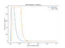
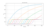
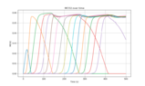
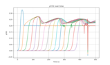
And here is the model/experimental data we were tuning to at the time: https://www.sciencedirect.com/science/article/abs/pii/S0009250909000852

Here are our model equations:
The gas phase mole balance
\begin{equation}
m_j\frac{dy_i}{dt} = \dot{m}_{j-1}(y_{j-1} - y_j) - M_{i,j}''A_s + y_{i,j}\sum\limits_{i=1}^{n_c} M_{j,z}''A_s
\end{equation}

The gas phase heat balance:
\begin{equation}
m_j C_{p,j}\frac{dT_g}{dt} = \dot{m}_{j-1}C_{p,j-1}(T_{j-1} - T_j) - q_{g,I,j}A_s
\end{equation}

The bed heat balance:
\begin{equation}
M_sC_{p,s,j}\frac{dT_b}{dt} = q_{I,b,j}A_s
\end{equation}

Solid phase mass balance:
\begin{equation}
\frac{dM_i}{dt} = M_i''A_s
\end{equation}

Mass flow out of a tank:
\begin{equation}
\dot{m}_{j} = \dot{m}_{j-1} + \frac{\rho_m}{T_g}A_C\Delta z\frac{dT}{dt} - \sum\limits_{i=1}^{n_c} M_{i,j}''A_s
\end{equation}

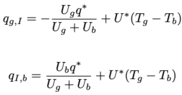
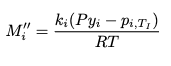
Here are our equations for ##M_{i,j}''##, ##q_{g,I}## and ##q_{I,b}##:
\begin{equation}
M_i'' = \frac{k_i(Py_i - p_{i,T_I})}{RT}
\end{equation}
\begin{equation}
q_{g,I} = -\frac{U_g q^*}{U_g+U_b} + U^*(T_g - T_b)
\end{equation}
\begin{equation}
q_{I,b} = \frac{U_b q^*}{U_g+U_b} + U^*(T_g - T_b)
\end{equation}
We also have correlations from BSL for the mass transfer coefficient ##k_i##, the fluid solid heat transfer coefficient ##h_{f,s}## and the sublimation pressure of CO2 ##p_{sub,co2}##:
\begin{equation}
h_{fs} = (2.19Re^{1/3} + 0.78Re^{0.619})Pr^{1/3}(\frac{k_g}{d_p})(\frac{\mu_{b,T_I}}{\mu_{0,T_I}})^{0.14}(1-\epsilon)
\end{equation}
\begin{equation}
k_{i} = (2.19Re^{1/3} + 0.78Re^{0.619})\frac{Sc^{1/3}}{d_p}D_{ab}(1-\epsilon_g)
\end{equation}
\begin{equation}
ln(\frac{P_{sub}}{P_t}) = \frac{T_t}{T}[a_1(1-\frac{T}{T_t)}+a_2(1-\frac{T}{T_t})^{1.9}+a_3(1-\frac{T}{T_t})^{2.9}]
\end{equation}

I'm not sure why the equation numbers are so high, but anyway -
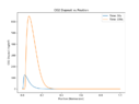
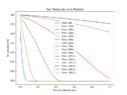
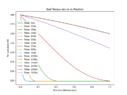
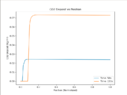
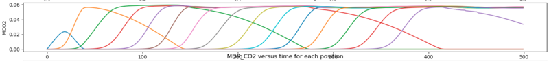
Right now since the output I'm getting is not as expected, I have set the mass and heat transfer coefficients to be constants. The only other big change is that we are no longer including ##H_2O## in this model, just a stream of Nitrogen and ##CO_2##.

Here are the constants, initial and boundary values as they are currently:
Constants:
U_b = 100
U_g = 50
cp_CO2 = 37
ki_CO2 = 5 * 10 ** -4 # mol/m2.s (I'm actually still not fully sure about this unit)

Initial values:
initial_co2_mole_fraction = 0.00
initial_co2_deposit = 0.0
initial_gas_temperature = 123.15
initial_bed_temperature = 123.15

Boundary Values:
molar_flow_in = 0.002
y_CO2_inlet = 0.2
T_inlet = 300
 

Attachments

  • Screenshot 2023-05-07 at 19.52.52.png
    Screenshot 2023-05-07 at 19.52.52.png
    14.8 KB · Views: 82
  • co2_unbounded.png
    co2_unbounded.png
    7.1 KB · Views: 85
  • position_versus_gas_temperature.png
    position_versus_gas_temperature.png
    15.6 KB · Views: 86
  • position_vs_bed_temperature.png
    position_vs_bed_temperature.png
    15.2 KB · Views: 102
  • co2_deposition_vs_position_kg.png
    co2_deposition_vs_position_kg.png
    8.8 KB · Views: 110
  • Screenshot 2023-05-07 at 19.59.13.png
    Screenshot 2023-05-07 at 19.59.13.png
    2.1 KB · Views: 96
  • Screenshot 2023-05-07 at 19.58.42.png
    Screenshot 2023-05-07 at 19.58.42.png
    2.6 KB · Views: 88
  • Screenshot 2023-05-07 at 19.58.25.png
    Screenshot 2023-05-07 at 19.58.25.png
    2.1 KB · Views: 83
  • Screenshot 2023-05-07 at 19.55.56.png
    Screenshot 2023-05-07 at 19.55.56.png
    3.1 KB · Views: 82
  • Screenshot 2023-05-07 at 19.55.05.png
    Screenshot 2023-05-07 at 19.55.05.png
    4.2 KB · Views: 83
  • #370
The output looks like this -
The output looks like this, for n = 200:
position_versus_gas_temperature.png

position_vs_bed_temperature.png


co2_unbounded.png


I wanted to incude this last plot showing every position (all 200) and how they behave over time. Clearly the CO2 mole fraction output isnt right. The other plots dont actually look too bad though.
co2_model_results_overview.png

In regards to the position vs temperature plots higher up, there doesnt seem to be any constant temperature zone which is present in Tuinier et al.

I apologise for the information dump but yes I would just like to open up dialogue here again as I found it hugely beneficial last time to have someone to have a back and forth with.

Is the above information sufficient or should I provide further info on this?

EDIT: One point I forgot to mention - in the gas/bed temperature vs position plots, I have printed time values. You can see that the temperature profile acually stops changing after a while and this is before the entirety of the bed has reached the inlet gas temperature
 
Last edited:
  • #371
casualguitar said:
The output looks like this -
The output looks like this, for n = 200:
View attachment 326119
View attachment 326120

View attachment 326121

I wanted to incude this last plot showing every position (all 200) and how they behave over time. Clearly the CO2 mole fraction output isnt right. The other plots dont actually look too bad though.
View attachment 326116
In regards to the position vs temperature plots higher up, there doesnt seem to be any constant temperature zone which is present in Tuinier et al.

I apologise for the information dump but yes I would just like to open up dialogue here again as I found it hugely beneficial last time to have someone to have a back and forth with.

Is the above information sufficient or should I provide further info on this?

EDIT: One point I forgot to mention - in the gas/bed temperature vs position plots, I have printed time values. You can see that the temperature profile acually stops changing after a while and this is before the entirety of the bed has reached the inlet gas temperature
What do the results look like if you run the model with the mass transfer coefficient set to zero?
 
  • #372
Chestermiller said:
What do the results look like if you run the model with the mass transfer coefficient set to zero?
Hi Chet, setting ki_CO2 = 0 and letting n=200 results in these plots:
Screenshot 2023-05-08 at 11.39.57.png


Screenshot 2023-05-08 at 11.40.33.png

Screenshot 2023-05-08 at 11.41.09.png

Screenshot 2023-05-08 at 11.41.21.png


The co2 mole fraction rises to 0.2 which is the inlet mole fraction, so this looks ok. There is no CO2 buildup on the bed as expected. The temperature profiles also generally look ok although there is no constant temeprature zone.

For reference, the h_desublimation_CO2 is set to 26,000 J/mol currently. Just now I tried setting it to 0 and 200,000, neither of which changed the temperature profiles appreciably
 
  • #373
casualguitar said:
Hi Chet, setting ki_CO2 = 0 and letting n=200 results in these plots:
View attachment 326147

View attachment 326148
View attachment 326149
View attachment 326150

The co2 mole fraction rises to 0.2 which is the inlet mole fraction, so this looks ok. There is no CO2 buildup on the bed as expected. The temperature profiles also generally look ok although there is no constant temeprature zone.

For reference, the h_desublimation_CO2 is set to 26,000 J/mol currently. Just now I tried setting it to 0 and 200,000, neither of which changed the temperature profiles appreciably
Why does the CO2 mole fraction rise so rapidly? What is the gas residence time in the bed?

I feel that the problem is related to the CO2 mass transfer, particularly when the conditions are such that there is no longer CO2 remaining deposited on the bed.
 
  • #374
Chestermiller said:
Why does the CO2 mole fraction rise so rapidly? What is the gas residence time in the bed?
I think due to the high flow. The inlet total molar flow for that plot was 0.002mol/s.

Here is a flow 10 times smaller. ##\dot{m_{in}}## = 0.0002mol/s
Screenshot 2023-05-08 at 12.40.25.png

Hmm to calculate gas residence time in the bed, could we do something like:
\begin{equation}
t_{residence} = \frac{L_{BED}}{v_{gas}}
\end{equation}

The velocity of the gas is:
\begin{equation}
v_{gas} = \frac{\dot{m_{in}}}{\rho A}
\end{equation}

where ##\dot{m_{in}}## is in mol/s, ##\rho## is in mol/m3 and A is in ##m^2##

For ##L_{BED}## = 0.3m:
##v_{gas}## = 0.0002/(36.36*0.00096) = 0.005m/s

Which gives a ##t_{residence}## value of ##52.63s##Just note at this point I'm using the bed dimensions, bed initial temperature, inlet gas temperature and inlet gas CO2 mole fraction from Tuinier et al. The inlet flow, mass transfer coefficient, and heat transfer coefficients are currently not the same. I can switch to the tuinier inlet mass flux now of 0.24kg/m2.s if the above is reasonable?
 
  • #375
There's something wrong with how the release of the CO2 from the bed is handled. If there is a driving force for removal but there is no CO2 left on the bed, the flow of CO2 from the bed to the gas has to be zero. That means that the mass balance equation for the CO2 in the gas has to allow for this. Is it?
 
  • #376
Chestermiller said:
There's something wrong with how the release of the CO2 from the bed is handled. If there is a driving force for removal but there is no CO2 left on the bed, the flow of CO2 from the bed to the gas has to be zero. That means that the mass balance equation for the CO2 in the gas has to allow for this. Is it?
No it doesn't allow for it. Right now the value can go below zero and does. Originally I had a conditional statement in the integrator that said "if the amount of CO2 in the bed goes below zero, set it to zero". Then I moved this statement to post-processing, so now I'm just plotting the CO2 deposition values that are above zero, but the solution from the integrator does contain negative values. Are either of these approaches ok, or should we somehow allow for it directly in the mass balance equation?

Right now the plots are unaffected by this (I think) since the mass transfer coefficient is zero thoughEdit: Sorry my apologies - I previously mentioned that there was no constant temperature zone. There is a constant temperature zone when the mass transfer coefficient is a non-zero value.

For reference, here's the CO2 buildup and other output when I dont post-process it to only show values greater than zero, when the mass-transfer coefficient is non-zero:
Screenshot 2023-05-09 at 16.27.52.png

The blue line in the CO2 buildup plot is position 0, the orange one is position 1, if we continue on this plot the other positions drop off to negative values similarly. The mole fraction of CO2 goes above the inlet molar concentration of CO2. The temperature plots also look unusual

Heres the gas temperature plot, just illustrating that the constant temperature zone is present:
Screenshot 2023-05-09 at 16.27.27.png


As you were saying there is likely an issue with how CO2 is released from the bed. How should we allow for the CO2 deposition value only being positive in the mole balance?

As mentioned, I am just post-processing the solution at the moment to remove the negative values. I can set the value to have a minimum value of zero inside the integrator though. Although I'm not sure if this is actually different to doing what I'm doing currently
 
Last edited:
  • #377
We must set ##\frac{dM_i}{dt}=0## if ##M_i\leq 0## and ##M_i^"<0##, which is equivalent to ##M_i\leq 0## and ##(Py_{i}-p_{i,T_I})<0##. I've been trying to figure out a simple way of doing this in coding without use of IF statements.
 
  • #378
There is an equivalent vectorised option in pythons numpy library called "where". Its just a vectorised if statement package though. I could replace the existing ##\frac{dM_i}{dt}## code lines (the boundary one and the internal nodes one) with something like this:

##\frac{dM_i}{dt} = np.where((M_i <= 0)## & ##(P * y_i - p_{i,T_I} < 0), 0, M_i'' * A_s)##

Which just says if the first two conditions are true then ##\frac{dM_i}{dt} = 0##, else ##\frac{dM_i}{dt} = M_i'' * A_s##

What is the reason that an IF statement isn't suitable here?

Edit: Just a note - heres the output with the above implemented. It does limit the CO2 deposited to a minimum of zero, but the mole fraction and temperature profiles are not right
Screenshot 2023-05-09 at 17.40.57.png


Just noting also that if the mass transfer coefficient is set to zero with the new code addition then the output looks reasonable again:
Screenshot 2023-05-09 at 17.45.18.png
 
Last edited:
  • #379
Is ##A_s## the bed surface area (m^2) per tank and ##M_I## the moles of CO2 deposited per tank? If so, pleases try to impose the following: If ##M_i<0.1 A_s## and ##M_{i}^"\leq 0##, reset ##M_i^"## to zero. This applies to the realistic flow rates.
 
Last edited:
  • #380
Chestermiller said:
Is ##A_s## the bed surface area (m^2) per tank and ##M_I## the moles of CO2 deposited per tank? If so, pleases try to impose the following: If ##M_i<0.1 A_s## and ##M_{i}^"\leq 0##, reset ##M_i^"## to zero. This applies to the realistic flow rates.
Yes. Here is the output when this is imposed:
##M_i<0.1 A_s## and ##M_{i}^"\leq 0##, reset ##M_i^"## to zero
Where ##A_s =A_c\Delta z a_s=\frac{6}{d_p}(1-\epsilon)A_c\Delta z = 0.0032m^2##, the molar flow is 0.002mol/s and k_i = 5 * 10 ** -4 mol/m2.s:
Screenshot 2023-05-10 at 12.02.04.png

Screenshot 2023-05-10 at 12.02.21.png

Screenshot 2023-05-10 at 12.02.35.png

Screenshot 2023-05-10 at 12.03.07.png

Screenshot 2023-05-10 at 12.03.32.png


Is the reason for the ##0.1A_s## constraint so that we dont run into any case where ##M_i## <0? In a case where ##M_i''## is large this may occur

Just a note - this is n=200. The output is very different for lower n (n=20 or so). I can clean up the plotting to plot say 10% of the total positions if needed
 

Attachments

  • Screenshot 2023-05-10 at 12.02.48.png
    Screenshot 2023-05-10 at 12.02.48.png
    8.9 KB · Views: 88
Last edited:
  • #381
casualguitar said:
Yes. Here is the output when this is imposed:

Where ##A_s =A_c\Delta z a_s=\frac{6}{d_p}(1-\epsilon)A_c\Delta z = 0.0032m^2##, the molar flow is 0.002mol/s and k_i = 5 * 10 ** -4 mol/m2.s:
View attachment 326285
View attachment 326286
View attachment 326287
View attachment 326289
View attachment 326290

Is the reason for the ##0.1A_s## constraint so that we dont run into any case where ##M_i## <0? In a case where ##M_i''## is large this may occur
Yes. Do you think 0.1 is too large. Why didn't you run the calculation for a realistic molar flow rate?

What are your thoughts on whether the new plots were closer to your expectations?
 
  • #382
Chestermiller said:
Yes. Do you think 0.1 is too large. Why didn't you run the calculation for a realistic molar flow rate?

What are your thoughts on whether the new plots were closer to your expectations?
No I think 0.1 is ok. Ah I was using a molar flow rate that fit the mass transfer coefficient. These two values affect the output quite a lot so if I change the molar flow I also need to adjust the mass transfer coefficient to get reasonable looking output.

The Tuinier et al reference uses 0.27kg/m2, which is 0.0083mol/s.

The Tuinier et al reference uses g = 1x10^-6 s/m. From post #233, the relationship between their g and our ##k_i## is:
\begin{equation}
k=\frac{1000RT}{M}g
\end{equation}
which gives ##k_{CO2}## = 0.047 for g = 1x10^-6.

Output using all of their values above looks like this (note the inlet temperature is 300K and the initial bed temperature is 123K):

The constant temperature zone is at approximately the right temperature, but the temperature seems to max out at around this temperature, rather than increase to the inlet gas temperature of 300K:
Screenshot 2023-05-11 at 14.47.34.png

The bed temperature seems to start at 0K actually, but ignoring this the rest of the temperature profile seems to be about the same as the gas temperature profile. I'll look into this 0K issue now
Screenshot 2023-05-11 at 14.47.52.png

The heat transfer profile at the inlet position (the blue one) does not look right, and the profile is very different to the internal node profiles:

Screenshot 2023-05-11 at 14.48.09.png


The CO2 buildup profile looks ok. We dont get the same max values as Tuinier but they dont specify the simulation conditions for their CO2 buildup plot:
Screenshot 2023-05-11 at 14.48.27.png


Investigating this 0K and heat transfer profile issue now
EDIT: That was a typo in how I was plotting the bed temperature. The ##Q_{BI}##/##Q_{IG}## issue still stands though
 

Attachments

  • Screenshot 2023-05-11 at 14.48.57.png
    Screenshot 2023-05-11 at 14.48.57.png
    26.6 KB · Views: 87
Last edited:
  • #383
Just one addition to the above - letting ki_CO2 = 0 results in output that looks as expected. So yes as you said its definitely related to how co2 is released from the bed:

Screenshot 2023-05-11 at 16.37.16.png

Screenshot 2023-05-11 at 16.37.48.png

The CO2 moves through the bed quickly as there is no desublimation:
Screenshot 2023-05-11 at 16.38.08.png
 
  • #384
The issue is with MDR (as you said previously). The molar desublimation rate at the inlet position does not trend towards zero as the other positions do. I will come back to this later this evening and see if the MDR function is implemented differently at the boundary
Screenshot 2023-05-11 at 16.43.25.png

Here's the function:
Screenshot 2023-05-11 at 16.45.30.png
 
  • #385
Hi Chet,

Just noting one other thing in regards to the CO2 flow through the bed (molar flow/molar holdup).

The molar flow out of the first tank is currently calculated as:
Screenshot 2023-05-12 at 23.47.25.png

which is the molar flow into tank 1 minus the total amount of CO2 deposited/released in that tank

Similarly, the molar flow out of the internal tanks is as follows:
Screenshot 2023-05-12 at 23.47.51.png


It looks ok to me but I'm just confirming this is correct

EDIT: I know why the heat transfer profiles (QGI and QIB) look the way they do. The gas/bed temperature plots get stuck at around the sublimation temperature, meaning that there will always be high heat transfer between the inlet gas and the first tank. The remaining tanks are at almost the same temperature as the first tank which is why we only see high heat transfer in the first one. That doesn't solve the problem but it does explain the QGI/QIB plots

EDIT 2: Whoops!! The molar flow out of the tank is wrong! I'm going to take a look at this tomorrow when I have a clear head
 
Last edited:
  • #386
Hi Chet,

Unfortunately the molar flow error didnt fix the output, although it did change it somewhat.

The molar flow out of a tank should have been defined as the below. It was previously this so I must have changed it somewhere along the way:
\begin{equation}
\dot{m}_j = \dot{m}_{j-1} + \frac{\rho_m \Delta z A_c}{T_g}\frac{dT}{dt} - (M_{CO_2}''*A_s)
\end{equation}

Further up in the code ##m_j## is defined as:
\begin{equation}
m_j = \frac{P}{RT_g}\epsilon A_C\Delta z
\end{equation}

So I now have:
\begin{equation}
\dot{m}_j = \dot{m}_{j-1} + \frac{\rho_m \Delta z A_c}{T_g}\frac{dT}{dt} - (M_{CO_2}''*A_s)
\end{equation}

which I've implemented as:
\begin{equation}
\dot{m}_j = \dot{m}_{j-1} + \frac{m_j \epsilon}{T_g}\frac{dT}{dt} - (M_{CO_2}''*A_s)
\end{equation}

Just posting this here in case I've done anything crazy there
 
  • #387
Hi Chet, looking further into the CO2 desublimation rate function, these are plots of temperature versus sublimation pressure (the gas-solid curve), and then temperature versus desublimation rate for a range of ##k_i## values, and ##y_{CO2}## = 0.2 (as it is in Tuinier et al).

Note that for the sublimation pressure curve, for temperature values above the triple point temperature (216K), i've used the liquid-vapour curve. Is there an alternative here? We could possibly say: if T is less than the triple point temperature, use the sublimation pressure curve, if T is greater than the triple point temeprature, let sublimation pressure = some large number?
Screenshot 2023-05-17 at 08.56.51.png
Screenshot 2023-05-17 at 09.00.00.png

Edit: just noting the simulation breaks if I let psubco2 = 1000000 for T > triple point temerpature
 
  • #388
Hi Chet, one more finding:

I ran a range of ##k_{CO2}## values as they have a very significant effect on all of the output. Here they are:

##k_{CO2}## = ##5*10^-4##:
Screenshot 2023-05-17 at 09.49.31.png
Screenshot 2023-05-17 at 09.49.48.png
Screenshot 2023-05-17 at 09.52.56.png


##k_{CO2}## = ##5*10^-5##:
Screenshot 2023-05-17 at 09.51.28.png
Screenshot 2023-05-17 at 09.51.43.png
Screenshot 2023-05-17 at 09.52.12.png

##k_{CO2}## = ##5*10^-6##:
Screenshot 2023-05-17 at 09.53.41.png
Screenshot 2023-05-17 at 09.53.59.png

Screenshot 2023-05-17 at 09.54.21.png

So yes again you were right with your original thought that CO2 sublimation isn't working correctly. Actually I've printed the CO2 sublimation pressure values versus temperature and as temperature gets to high values the sublimation pressure does too, meaning that we should see high sublimation rates of CO2, but we dont (the CO2 deposition plot is horizontal at high temperatures).
 

Attachments

  • Screenshot 2023-05-17 at 09.55.11.png
    Screenshot 2023-05-17 at 09.55.11.png
    7.7 KB · Views: 100
  • #389
My apologies for the long-winded posts (my head is a bit fried!). The first plot below is completely at odds with the second one is it not? These plots are from the same simulation
Screenshot 2023-05-17 at 10.19.09.png


Screenshot 2023-05-17 at 10.20.15.png
 
  • #390
Hi Chet,

Output is looking better now. Only issue really is that we're producing a lot more solid CO2. The profiles look ok though.

I reverted back to an older approach we had, where we used something like their "fudge factor". I also put in the previous correlation for ##k_{CO2}##.

The fudge factor looks like this and only applies for sublimation (not desublimation):
if ##P*y_{CO2}## < ##P_{sub,CO2}##:
##M_{CO2}''## = ##M_{CO2}''##*##(\frac{M_{CO2}}{M_{CO2}+0.1})##

Tuinier uses 0.1 as their fudge factor. I'm using 0.1 also currently. We previously also discussed converting this 0.1 to a value suitable for us (different units), like this:
factor = 0.1*1000*A_C*dz/mW_CO2

As we're now calculating ##k_{CO2}##, we can no longer use this as a tuning parameter, unless I'm wrong. I'm wondering if we can instead use this fudge factor to tune the amount of CO2 produced?

Here's the output from the above. Note the output is a bit rough looking because I have used n=15. The the simulation takes a lot longer to run now so I'll increase this again once we're happy with the output:

Gas temperature profile shows the constant temperature zone:
Screenshot 2023-05-17 at 16.36.00.png


The amount of CO2 on the bed in kg/m3. Tuinier et al had values closer to 50kg/m3 for 50s and 150s:
Screenshot 2023-05-17 at 16.37.45.png


Lastly, ##y_{CO2}## for each position. Each position does level out at 0.2 which is the inlet concentration. There is a bit of fluctuation but this is possibly down to the sublimation process (I'll check this):
Screenshot 2023-05-17 at 16.38.39.png


If this looks ok to you, do you think it is reasonable to use the "factor" to tune the amount of CO2 on the bed to Tuinier et al?

EDIT: If I take out the fudge factor and run it, the output looks like it did before (incorrect). I didn't think the fudge factor would have such an impact!
 

Attachments

  • Screenshot 2023-05-17 at 14.07.29.png
    Screenshot 2023-05-17 at 14.07.29.png
    17.3 KB · Views: 116
  • Screenshot 2023-05-17 at 14.06.54.png
    Screenshot 2023-05-17 at 14.06.54.png
    33.8 KB · Views: 90
  • Screenshot 2023-05-17 at 14.06.23.png
    Screenshot 2023-05-17 at 14.06.23.png
    30.8 KB · Views: 113
  • Screenshot 2023-05-17 at 14.05.50.png
    Screenshot 2023-05-17 at 14.05.50.png
    9.7 KB · Views: 104
Last edited:

Similar threads

Replies
454
Views
27K
  • · Replies 2 ·
Replies
2
Views
2K
  • · Replies 6 ·
Replies
6
Views
2K
  • · Replies 0 ·
Replies
0
Views
1K
  • · Replies 1 ·
Replies
1
Views
1K
Replies
5
Views
1K
  • · Replies 25 ·
Replies
25
Views
3K
Replies
26
Views
5K
Replies
31
Views
3K
  • · Replies 8 ·
Replies
8
Views
3K