Optimizing Orbits with Runge-Kutta-Nyström Method

  • Thread starter Dmalyuta
  • Start date
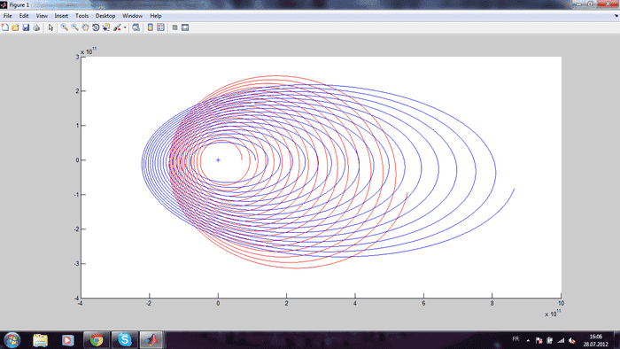
In summary, the conversation is about a problem with a simulation program written in Matlab that is trying to simulate the orbits of Mercury and Venus around the Sun. The issue is that the planets are spinning out of orbit and not staying in an ellipse. The person is asking for help in finding the mistake in their code that is causing this bizarre motion. The code is provided for reference.
  • #1
Dmalyuta
7
0
Hi all,

I'm using Matlab to try and smulate the orbits of Mercury and Venus aroudn the Sun, allowing all three to disturbe each others' orbits.

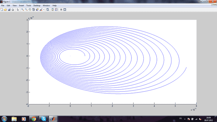
However, I am constantly running into this problem- all of my orbits look like in the pictures below- in effect, the planets spin out of orbit and will not stay in one ellipse. Even when I Venus out of the equation, mercury still displays this wild behavior.

This is obviosly the result of a problem in the code I've written for this simulation; my question si whether someone could explain to me for what reason such bizarre motion would result (what force is missing, etc.?) so that I can start looking in the right places in my code. For reference, the code I wrote is as follows. For only Sun and Mercury:

Code:
% Mapping planet coordinates for 3 bodies- Sun, Mercury, Venus

clear
clf

%% Asking user to input some information and defining some constants

tim=10000;
interva=0.3;

G=6.67384e-11;

%% Sun initial coordinates

M_S=1.989e+30; % mass of sun
x(1,1)=0.0; % x-coordinate. (a,b) where a is the planet number (Sun is #1) and b is the time interval number (1 means time=0s)
y(1,1)=0.0;
V_x(1,1)=0.0; % velocity in x-direction
V_y(1,1)=0.0; % velocity in y-direction

%% Mercury initial coordinates

M_M=3.3e+23; % mass of mercury
x(2,1)=6.98e+10; % note that here a=2, which is mercury's number from the Sun. x-coordinate derived from planet's aphelion
y(2,1)=0.0; % all planets in my simulation start from x-axis
V_x(2,1)=0.0;
V_y(2,1)=38860; % note that all planets start from minimum velocity as such is the case at the aphelion (furthest) position from the sun

%% Venus initial coordinates

M_V=4.87e+24; % mass of venus
x(3,1)=1.09e+11;
y(3,1)=0.0;
V_x(3,1)=0.0;
V_y(3,1)=34790;

%% We now run a loop which will drop out coordiantes of planet positions at different times

timeend=tim*24*3600;
interval=interva*24*3600;

cell=1;

for iter=0:interval:timeend
    
    for i=1:2
        
        switch i
            
            case 1
                
                r_SM=sqrt((x(2,cell)-x(1,cell))^2+(y(2,cell)-y(1,cell))^2);
                r_SV=sqrt((x(3,cell)-x(1,cell))^2+(y(3,cell)-y(1,cell))^2);
                
                a_x(1,cell)=-(G*M_M*(x(1,cell)-x(2,cell)))/(r_SM^3);
                a_y(1,cell)=-(G*M_M*(y(1,cell)-y(2,cell)))/(r_SM^3);
                
                V_x(1,cell+1)=V_x(1,cell)+interval*a_x(1,cell);
                V_y(1,cell+1)=V_y(1,cell)+interval*a_y(1,cell);
                                
                x(1,cell+1)=x(1,cell)+interval*V_x(1,cell);
                y(1,cell+1)=y(1,cell)+interval*V_y(1,cell);
                
            case 2
                
                r_SM=sqrt((x(2,cell)-x(1,cell))^2+(y(2,cell)-y(1,cell))^2);
                r_MV=sqrt((x(3,cell)-x(2,cell))^2+(y(3,cell)-y(2,cell))^2);
                               
                a_x(2,cell)=-(G*M_S*(x(2,cell)-x(1,cell)))/(r_SM^3);
                a_y(2,cell)=-(G*M_S*(y(2,cell)-y(1,cell)))/(r_SM^3);
                
                V_x(2,cell+1)=V_x(2,cell)+interval*a_x(2,cell);
                V_y(2,cell+1)=V_y(2,cell)+interval*a_y(2,cell);
                
                x(2,cell+1)=x(2,cell)+interval*V_x(2,cell);
                y(2,cell+1)=y(2,cell)+interval*V_y(2,cell);
                
        end
        
    end
    
    cell=cell+1;
    
end

hold on

for i=1:2
    
    plot(x(i,:),y(i,:))
    
end

hold off

For Sun, Mercury, and Venus:

Code:
% Mapping planet coordinates for 3 bodies- Sun, Mercury, Venus

clear
clf

%% Asking user to input some information and defining some constants

tim=10000;
interva=0.3;

G=6.67384e-11;

%% Sun initial coordinates

M_S=1.989e+30; % mass of sun
x(1,1)=0.0; % x-coordinate. (a,b) where a is the planet number (Sun is #1) and b is the time interval number (1 means time=0s)
y(1,1)=0.0;
V_x(1,1)=0.0; % velocity in x-direction
V_y(1,1)=0.0; % velocity in y-direction

%% Mercury initial coordinates

M_M=3.3e+23; % mass of mercury
x(2,1)=6.98e+10; % note that here a=2, which is mercury's number from the Sun. x-coordinate derived from planet's aphelion
y(2,1)=0.0; % all planets in my simulation start from x-axis
V_x(2,1)=0.0;
V_y(2,1)=38860; % note that all planets start from minimum velocity as such is the case at the aphelion (furthest) position from the sun

%% Venus initial coordinates

M_V=4.87e+24; % mass of venus
x(3,1)=1.09e+11;
y(3,1)=0.0;
V_x(3,1)=0.0;
V_y(3,1)=34790;

%% We now run a loop which will drop out coordiantes of planet positions at different times

timeend=tim*24*3600;
interval=interva*24*3600;

cell=1;

for iter=0:interval:timeend
    
    for i=1:3
        
        switch i
            
            case 1
                
                r_SM=sqrt((x(2,cell)-x(1,cell))^2+(y(2,cell)-y(1,cell))^2);
                r_SV=sqrt((x(3,cell)-x(1,cell))^2+(y(3,cell)-y(1,cell))^2);
                
                a_x(1,cell)=-(G*M_M*(x(1,cell)-x(2,cell)))/(r_SM^3)+-(G*M_V*(x(1,cell)-x(3,cell)))/(r_SV^3);
                a_y(1,cell)=-(G*M_M*(y(1,cell)-y(2,cell)))/(r_SM^3)+-(G*M_V*(y(1,cell)-y(3,cell)))/(r_SV^3);
                
                V_x(1,cell+1)=V_x(1,cell)+interval*a_x(1,cell);
                V_y(1,cell+1)=V_y(1,cell)+interval*a_y(1,cell);
                                
                x(1,cell+1)=x(1,cell)+interval*V_x(1,cell);
                y(1,cell+1)=y(1,cell)+interval*V_y(1,cell);
                
            case 2
                
                r_SM=sqrt((x(2,cell)-x(1,cell))^2+(y(2,cell)-y(1,cell))^2);
                r_MV=sqrt((x(3,cell)-x(2,cell))^2+(y(3,cell)-y(2,cell))^2);
                               
                a_x(2,cell)=-(G*M_S*(x(2,cell)-x(1,cell)))/(r_SM^3)+-(G*M_V*(x(2,cell)-x(3,cell)))/(r_SV^3);
                a_y(2,cell)=-(G*M_S*(y(2,cell)-y(1,cell)))/(r_SM^3)+-(G*M_V*(y(2,cell)-y(3,cell)))/(r_SV^3);
                
                V_x(2,cell+1)=V_x(2,cell)+interval*a_x(2,cell);
                V_y(2,cell+1)=V_y(2,cell)+interval*a_y(2,cell);
                
                x(2,cell+1)=x(2,cell)+interval*V_x(2,cell);
                y(2,cell+1)=y(2,cell)+interval*V_y(2,cell);
                
            case 3
                
                r_SV=sqrt((x(3,cell)-x(1,cell))^2+(y(3,cell)-y(1,cell))^2);
                r_MV=sqrt((x(3,cell)-x(2,cell))^2+(y(3,cell)-y(2,cell))^2);
                
                a_x(3,cell)=-(G*M_S*(x(3,cell)-x(1,cell)))/(r_SM^3)+-(G*M_M*(x(3,cell)-x(2,cell)))/(r_SV^3);
                a_y(3,cell)=-(G*M_S*(y(3,cell)-y(1,cell)))/(r_SM^3)+-(G*M_M*(y(3,cell)-y(2,cell)))/(r_SV^3);
                
                V_x(3,cell+1)=V_x(3,cell)+interval*a_x(3,cell);
                V_y(3,cell+1)=V_y(3,cell)+interval*a_y(3,cell);
                                
                x(3,cell+1)=x(3,cell)+interval*V_x(3,cell);
                y(3,cell+1)=y(3,cell)+interval*V_y(3,cell);
                
        end
        
    end
    
    cell=cell+1;
    
end

hold on

plot(x(1,:),y(1,:),'+')
plot(x(2,:),y(2,:),'r')
plot(x(3,:),y(3,:),'b')

hold off

yO4lX.png


Iczfq.png
 
Physics news on Phys.org
  • #2
Welcome to PF!

The acceleration you calculate in each step should not be accumulated, that is, you should have "=" and not "=-" for the lines that calculate acceleration.

In addition, you are using the very simple Euler integration [1] which will introduce false energy into the system. A better approach would be to use Leapfrog or a something method [2].

I have not made a detailed examination of your code, so I may easily have missed any other errors.

[1] http://en.wikipedia.org/wiki/Euler_method
[2] http://en.wikipedia.org/wiki/Leapfrog_method
 
  • #3
Filip Larsen said:
The acceleration you calculate in each step should not be accumulated, that is, you should have "=" and not "=-" for the lines that calculate acceleration.
That's not the problem. This is not accumulating. That would be -=. His "=-" is the same as "acc = -(computation)".

In addition, you are using the very simple Euler integration [1] which will introduce false energy into the system.
That's not the problem, either. He's using symplectic Euler, not Euler's method. Admittedly there are far better techniques, but symplectic Euler is an okay start. (Aside: Leapfrog is barely a step above symplectic Euler. There are far, far better.)The problem is that the accelerations are being computed sequentially. The accelerations need to be computed all at once, followed by state propagation.
 
  • #4
Could you please use simpler language in explaining that last problem about calculating accelerations all at once? I'm just trying to make sense of why the heck the planets would constantly be gaining energy and be moving into a higher orbit- there is nothing in my code which would imply that. Otherwise, it might be a problem of me loosing some force when the planets go below the x-axis; but then again, where in my code am I loosing that force??

PS. The code is extrapolated from Feynman's "Mechanics 1"- he described a numerical calculation for the sun and a planet (2 bodies) and touched upon 3 bodies (which is reflected in my code).
 
  • #5
You need to calculate all the accelerations before you update the position of the objects.

Code:
                r_SM=sqrt((x(2,cell)-x(1,cell))^2+(y(2,cell)-y(1,cell))^2);
                r_SV=sqrt((x(3,cell)-x(1,cell))^2+(y(3,cell)-y(1,cell))^2);
                
                a_x(1,cell)=-(G*M_M*(x(1,cell)-x(2,cell)))/(r_SM^3)+-(G*M_V*(x(1,cell)-x(3,cell)))/(r_SV^3);
                a_y(1,cell)=-(G*M_M*(y(1,cell)-y(2,cell)))/(r_SM^3)+-(G*M_V*(y(1,cell)-y(3,cell)))/(r_SV^3);

                r_SM=sqrt((x(2,cell)-x(1,cell))^2+(y(2,cell)-y(1,cell))^2);
                r_MV=sqrt((x(3,cell)-x(2,cell))^2+(y(3,cell)-y(2,cell))^2);
                               
                a_x(2,cell)=-(G*M_S*(x(2,cell)-x(1,cell)))/(r_SM^3)+-(G*M_V*(x(2,cell)-x(3,cell)))/(r_SV^3);
                a_y(2,cell)=-(G*M_S*(y(2,cell)-y(1,cell)))/(r_SM^3)+-(G*M_V*(y(2,cell)-y(3,cell)))/(r_SV^3);
                
                r_SV=sqrt((x(3,cell)-x(1,cell))^2+(y(3,cell)-y(1,cell))^2);
                r_MV=sqrt((x(3,cell)-x(2,cell))^2+(y(3,cell)-y(2,cell))^2);
                
                a_x(3,cell)=-(G*M_S*(x(3,cell)-x(1,cell)))/(r_SM^3)+-(G*M_M*(x(3,cell)-x(2,cell)))/(r_SV^3);
                a_y(3,cell)=-(G*M_S*(y(3,cell)-y(1,cell)))/(r_SM^3)+-(G*M_M*(y(3,cell)-y(2,cell)))/(r_SV^3);
                
                V_x(1,cell+1)=V_x(1,cell)+interval*a_x(1,cell);
                V_y(1,cell+1)=V_y(1,cell)+interval*a_y(1,cell);

                V_x(2,cell+1)=V_x(2,cell)+interval*a_x(2,cell);
                V_y(2,cell+1)=V_y(2,cell)+interval*a_y(2,cell);

                V_x(3,cell+1)=V_x(3,cell)+interval*a_x(3,cell);
                V_y(3,cell+1)=V_y(3,cell)+interval*a_y(3,cell);
                                
                x(1,cell+1)=x(1,cell)+interval*V_x(1,cell);
                y(1,cell+1)=y(1,cell)+interval*V_y(1,cell);
                
                x(2,cell+1)=x(2,cell)+interval*V_x(2,cell);
                y(2,cell+1)=y(2,cell)+interval*V_y(2,cell);
                
                x(3,cell+1)=x(3,cell)+interval*V_x(3,cell);
                y(3,cell+1)=y(3,cell)+interval*V_y(3,cell);

(I don't think your "for i=1:3", "switch i", and "case" statements do anything useful here).
 
  • #6
D H said:
That's not the problem. [...] He's using symplectic Euler, not Euler's method.

Good thing you are more awake than I apparently was :rolleyes: Hope the OP didn't get too confused about my wild shots there ...
 
  • #7
D H said:
The problem is that the accelerations are being computed sequentially. The accelerations need to be computed all at once, followed by state propagation.
I don't think that's it either. They are effectively calculated in parallel. The new acceleration is stored in cell+1. This isn't used until the next time around the loop.

It could be just accumulation of error through using finite intervals. Is it better if you reduce the interval size? That's always a useful test - reduce the interval size until it stops having a discernible effect on the result. A possible improvement is to use the average of the old and new accelerations when updating the velocities, and the average of old and new velocities when updating positions. This is roughly equivalent to reducing the interval size a bit.
 
  • #8
haruspex, I don't think this is accumulation of error as I used the same method to simulate the motion of just the Sun and mercury without Venus and Mercury's orbit was perfectly fine.

I think we should look into the signs of my calculated forces/accelerations in each quadrant when the x and y-coordinate signs change. I tried but I am blinded by the fact that I wrote the code, so it's harder for me to fidn the error than if somebody took a shot at it...
 
  • #9
haruspex said:
I don't think that's it either. They are effectively calculated in parallel. The new acceleration is stored in cell+1. This isn't used until the next time around the loop.
You're right, and so was Filip Larsen in post #2. The OP is using plain old Euler, which spirals out.

Even if the OP used the best integrator in the world, the ellipses would still move. The reason is that the Sun is starting with zero velocity. This makes the center of mass of the system as a whole have a non-zero velocity, about 6.45 milimeters per second, or 203 km/year, in the OP's first example of the Sun and Mercury.
 
  • #10
I re-wrote the code, and am still getting this bizarre effect. Here is the new code:

Code:
%% The Three Body Problem

clear
clf

%% Asking user to input some information and defining some constants

tim=10000;
interva=0.3;

G=6.67384e-11;

%% Sun initial coordinates

M(1)=1.989e+30; % mass of sun
x(1,1)=0.0; % x-coordinate. (a,b) where a is the planet number (Sun is #1) and b is the time interval number (1 means time=0s)
y(1,1)=0.0;
V_x(1,1)=0.0; % velocity in x-direction
V_y(1,1)=0.0; % velocity in y-direction

%% Mercury initial coordinates

M(2)=3.3e+23; % mass of mercury
x(2,1)=6.98e+10; % note that here a=2, which is mercury's number from the Sun. x-coordinate derived from planet's aphelion
y(2,1)=0.0; % all planets in my simulation start from x-axis
V_x(2,1)=0.0;
V_y(2,1)=38860; % note that all planets start from minimum velocity as such is the case at the aphelion (furthest) position from the sun

%% Venus initial coordinates

M(3)=4.87e+24; % mass of venus
x(3,1)=1.09e+11;
y(3,1)=0.0;
V_x(3,1)=0.0;
V_y(3,1)=34790;

%% We now run a loop which will drop out coordinates of planet positions at different times

timeend=tim*24*3600;
interval=interva*24*3600;

cell=1;

for time=0:interval:timeend
    
    for i=1:3
        
        switch i
            
            case 1
            
                % Calculate the next x-coordinate

                r(i,2,cell)=sqrt((x(i,cell)-x(2,cell))^2+(y(i,cell)-y(2,cell))^2);
                r(i,3,cell)=sqrt((x(i,cell)-x(3,cell))^2+(y(i,cell)-y(3,cell))^2);

                a_x(i,cell)=-(G*M(2)*(x(i,cell)-x(2,cell)))/(r(i,2,cell)^3)+-(G*M(3)*(x(i,cell)-x(3,cell)))/(r(i,3,cell)^3);
            
                V_x(i,cell+1)=V_x(i,cell)+interval*a_x(i,cell);
                
                x(i,cell+1)=x(i,cell)+interval*V_x(i,cell);
                
                % Calculate the next y-coordinate
                
                a_y(i,cell)=-(G*M(2)*(y(i,cell)-y(2,cell)))/(r(i,2,cell)^3)+-(G*M(3)*(y(i,cell)-y(3,cell)))/(r(i,3,cell)^3);
            
                V_y(i,cell+1)=V_y(i,cell)+interval*a_y(i,cell);
                
                y(i,cell+1)=y(i,cell)+interval*V_y(i,cell);
                
            case 2
                
                % Calculate the next x-coordinate

                r(i,1,cell)=sqrt((x(i,cell)-x(1,cell))^2+(y(i,cell)-y(1,cell))^2);
                r(i,3,cell)=sqrt((x(i,cell)-x(3,cell))^2+(y(i,cell)-y(3,cell))^2);

                a_x(i,cell)=-(G*M(1)*(x(i,cell)-x(1,cell)))/(r(i,1,cell)^3)+-(G*M(3)*(x(i,cell)-x(3,cell)))/(r(i,3,cell)^3);
            
                V_x(i,cell+1)=V_x(i,cell)+interval*a_x(i,cell);
                
                x(i,cell+1)=x(i,cell)+interval*V_x(i,cell);
                
                % Calculate the next y-coordinate
                
                a_y(i,cell)=-(G*M(1)*(y(i,cell)-y(1,cell)))/(r(i,1,cell)^3)+-(G*M(3)*(y(i,cell)-y(3,cell)))/(r(i,3,cell)^3);
            
                V_y(i,cell+1)=V_y(i,cell)+interval*a_y(i,cell);
                
                y(i,cell+1)=y(i,cell)+interval*V_y(i,cell);
                
            case 3
                
                % Calculate the next x-coordinate

                r(i,2,cell)=sqrt((x(i,cell)-x(2,cell))^2+(y(i,cell)-y(2,cell))^2);
                r(i,1,cell)=sqrt((x(i,cell)-x(1,cell))^2+(y(i,cell)-y(1,cell))^2);

                a_x(i,cell)=-(G*M(2)*(x(i,cell)-x(2,cell)))/(r(i,2,cell)^3)+-(G*M(1)*(x(i,cell)-x(1,cell)))/(r(i,1,cell)^3);
            
                V_x(i,cell+1)=V_x(i,cell)+interval*a_x(i,cell);
                
                x(i,cell+1)=x(i,cell)+interval*V_x(i,cell);
                
                % Calculate the next y-coordinate
                
                a_y(i,cell)=-(G*M(2)*(y(i,cell)-y(2,cell)))/(r(i,2,cell)^3)+-(G*M(1)*(y(i,cell)-y(1,cell)))/(r(i,1,cell)^3);
            
                V_y(i,cell+1)=V_y(i,cell)+interval*a_y(i,cell);
                
                y(i,cell+1)=y(i,cell)+interval*V_y(i,cell);

        end
        
    end
    
    cell=cell+1;
    
end

hold on

plot(x(1,:),y(1,:),'+');
plot(x(2,:),y(2,:),'r');
plot(x(3,:),y(3,:),'b');

hold off

And here is a picture of the resulting orbits:
2AciZ.png


I am thinking that perhaps the planets spin out of orbit because the sun is allowed to move around? If you zoom into the Sun, you get this pattern for its motion:
SWlZ2.png


Note how much it moves (7 orders of magnitude in the y-direction!); but then again, the real sun is allowed to move and the planets don't spin out of orbit- so what's the problem??! This is really starting to annoy me...
 
  • #11
The problem may be that your initial conditions are such that the total momentum of the system is not zero. The center of mass is in motion. If you want nice closed trajectories you need to calculate in the center of mass system or arrange the initial conditions so that the speed of the CM is zero in the system of reference used.
Maybe you do calculate in the CM? I did not go through your code in detail.
 
  • #12
D H said:
Even if the OP used the best integrator in the world, the ellipses would still move. The reason is that the Sun is starting with zero velocity. This makes the center of mass of the system as a whole have a non-zero velocity, about 6.45 milimeters per second, or 203 km/year, in the OP's first example of the Sun and Mercury.

Yes, you are correct. However, that will cause the simulation to creep, not spiral. This effect is much more noticable when doing a simulation of the Earth moon system. When I do a simulation of the Earth moon system I must give the moon a positive initial velocity and the Earth a negative initial velocity, otherwise it will creep. All bodies should have velocities relatve to the center of mass of the system (as nasu pointed out).

I cannot find a problem with this code. however, I am not very familiar with Matlab. So I don't know what's causing this. It does look like an accumulative problem, but I don't see it in the code. I do agree with AlephZero, that your use of the "I" loop is ineffective. However, I don't think that has anything to do with this problem. But it may be something you will want to fix if you decide to use more n-bodies.
 
  • #13
Dmalyuta said:
I re-wrote the code, and am still getting this bizarre effect. Here is the new code:

Code:
                a_x(i,cell)=-(G*M(2)*(x(i,cell)-x(2,cell)))/(r(i,2,cell)^3)+-(G*M(3)*(x(i,cell)-x(3,cell)))/(r(i,3,cell)^3);
            
                V_x(i,cell+1)=V_x(i,cell)+interval*a_x(i,cell);
                
                x(i,cell+1)=x(i,cell)+interval*V_x(i,cell);
You are still using Euler's method, and you are still intermixing calculations of accelerations and using them for propagation, and you probably still have the Sun starting with zero velocity.

Don't use Euler's method. It will give bad results. It is important to learn Euler's method because this method is the basis for many integration techniques. However, because the results are inevitably poor, it is also important to learn that it is best to not use this method.

Don't intermingle the calculations of accelerations and using them for propagation. It's not hurting you here, but that's only because you are using Euler's method. You can't get away with this for more advanced techniques. Calculate all of your accelerations before you do anything with them. One good way to do this is to put your acceleration computations (all of them) in a separate subroutine.

Don't make the Sun's initial velocity zero. You need to make the velocity of the system center of mass zero. If you don't the system as a whole will drift with this velocity.
Dmalyuta said:
This is really starting to annoy me...
Your wide images are starting to annoy me. Scale them down to a reasonable width. 800 pixels or 640 pixels are a good values. Don't go wider than 800, please.
 
Last edited:
  • #14
Thank you for the help. I took a shot at something, and now I feel stupid for having spent so much of your and my own time on this spiral dilemma- the problem was in, like many of you said, the method i was using and, in particular, the interval I was using. With 0.3 days, I get the spiral effect like in the pictures in above posts; I now changed to 0.001 days, and now I get this graph:
mMCoU.png

Now, my next question is- which method do you suggest I use which will give me a much more accurate result with an interval larger than 0.001 days (which takes a long time for my computer to compute!)?

Thank you!
 
  • #15
Dmalyuta said:
Now, my next question is- which method do you suggest I use which will give me a much more accurate result with an interval larger than 0.001 days (which takes a long time for my computer to compute!)?
First off, did you try symplectic Euler? In a nutshell, you use the updated velocity to propagate position rather than the pre-update velocity. It seems wrong, but it has a solid mathematical basis.

Filip gave you pointers to leapfrog, which has a number of variants. Another simple technique is velocity verlet. Leapfrog and verlet integration are often used in simulations of a large number (thousands or more) of bodies. These techniques aren't used so much because they're good; they're only good when compared to Euler / symplectic Euler. They're used because of how they come close to conserving energy.

There's an almost inescapable tradeoff here between long-term and short-term accuracy. Energy and angular momentum must be conserved to attain long-term accuracy (many million years for solar system simulations, or much shorter span for galactic-scale simulations). However, the techniques that do conserve energy / angular momentum are low order and only conserve these quantities approximately. (Better said: They preserve something that is a close analog to energy.)

If you want short-term accuracy you need to use higher order techniques. (Note that short term can mean millions of years with a good technique.) A good place to start is fourth order Runge Kutta. This technique takes four internal steps to achieve the desired external step size. Another approach is to take advantage of accelerations and velocities from previous time steps as well as the current step. This leads to the Adams-Bashforth-Moulton family of techniques. Gauss Jackson is very similar to the ABM family, but it is very hairy. Yet another approach is to specify a very long time step and let the integration technique split this up however it sees fit. You use Matlab; this is exactly what ode45() does.

A very different approach is to integrate something other than cartesian position and velocity. The orbits of the planets are very close to being ellipses. So propagate a reference ellipse, and compute your actual state as a perturbation from this. This approach was used with the Apollo missions. An alternative is to represent state as orbital elements rather than position and velocity and compute the time derivatives of these orbital elements. These derivatives are called the planetary equations of motion. There are a number of these, depending on which orbital elements one is using. A similar approach is to use quaternions to represent planetary state via the Karhunen–Loève transform.
 
  • #16
I came across this problem a while ago and ended up using the methods of Quinlan and Tremaine (1990). You basically find the new position as a function of the previous n positions/velocities/accelerations. A good approach is to generate the first few positions using a leapfrog method with very small timestep, then switch to a symmetric multistep method once you've gathered enough consecutive positions, increasing the length of the timestep to make it run faster.

They generally seem to conserve energy fairly well, and are fairly easy to code.

http://adsabs.harvard.edu/full/1990AJ...100.1694Q
 
  • #17
Dmalyuta said:
Now, my next question is- which method do you suggest I use which will give me a much more accurate result with an interval larger than 0.001 days (which takes a long time for my computer to compute!)?

I prefer Runge-Kutta-Nyström:

http://theory.gsi.de/~vanhees/faq/gravitation/node62.html

This is your example with an interval of 10 days:

http://tinyurl.com/cod5qwy
 

Related to Optimizing Orbits with Runge-Kutta-Nyström Method

1. What is the Three-Body Problem?

The Three-Body Problem is a mathematical problem that involves predicting the motion of three celestial bodies that are influenced by their mutual gravitational attraction. It is one of the oldest problems in physics, dating back to Newton's laws of motion in the 17th century.

2. Why is the Three-Body Problem significant?

The Three-Body Problem is significant because it has been proven to be mathematically unsolvable. This means that there is no exact formula or equation that can accurately predict the motion of three bodies in space, making it a challenging and important problem in the field of physics and astronomy.

3. What are some real-world applications of the Three-Body Problem?

The Three-Body Problem has many applications in the field of astrodynamics, such as predicting the trajectories of spacecraft or satellites in orbit around multiple bodies. It is also used in the study of celestial mechanics and the formation of planetary systems.

4. Are there any solutions or approximations to the Three-Body Problem?

While there is no exact solution to the Three-Body Problem, there are various numerical methods and approximations that can be used to make predictions about the motion of three bodies. These include the n-body simulation method and the restricted three-body problem, which simplifies the problem by assuming one of the bodies is much smaller than the other two.

5. How does the Three-Body Problem relate to chaos theory?

The Three-Body Problem is closely related to chaos theory, as the motion of three bodies can become chaotic and unpredictable over time. This is due to the sensitive dependence on initial conditions, meaning that even small changes in the starting positions or velocities of the bodies can lead to vastly different outcomes.

Similar threads

  • Classical Physics
Replies
2
Views
810
  • Classical Physics
Replies
4
Views
1K
Replies
61
Views
899
  • Mechanics
Replies
18
Views
2K
  • Classical Physics
Replies
6
Views
2K
  • Engineering and Comp Sci Homework Help
Replies
3
Views
1K
  • Engineering and Comp Sci Homework Help
Replies
6
Views
883
  • Introductory Physics Homework Help
Replies
5
Views
3K
Replies
1
Views
9K
Replies
7
Views
1K
Back
Top