Disappearing energy from a series connection of coupled oscillators

AI Thread Summary
The discussion focuses on issues related to energy calculations in a system of coupled oscillators modeled in Matlab. The user reports a significant loss of energy during simulations despite having set up the system with constant stiffness and no damping effects. Concerns are raised about the integration method used for the dynamic equations, suggesting that Euler's method may introduce systematic errors leading to energy non-conservation. The user confirms that the stiffness is fixed at the beginning of the simulation and that the code for calculating energy may contain errors. The conversation emphasizes the importance of reviewing the integration approach and the potential impact of variable stiffness on energy calculations.
bcolson
Messages
3
Reaction score
0
I have been having trouble getting the calculation of energy for a chain of coupled oscillators to come out correctly. The program was run in Matlab and is intended to calculate the energy of a system of connected Hooke's law oscillators. Right now there is only stiffness and no dampening effects or force functions.

Half of the system has stiffness 1 the other half has variable stiffness.
When I ran the program to calculate the energy of a system where stiffness = 1, 4 total masses, no kinetic energy or potential energy except on mass #1 and plotted out the energy vs time a large chunk of energy disappeared.
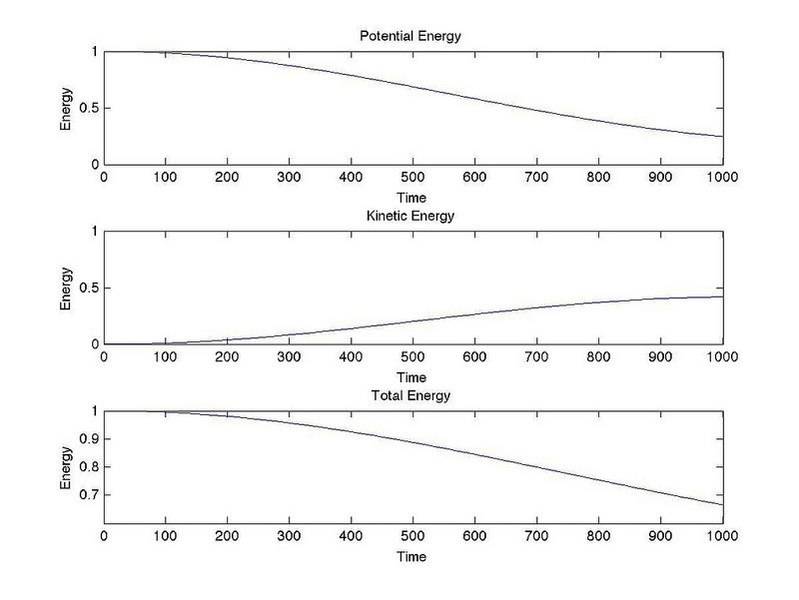
29712798611_8cac9764f1_c.jpg
the definitions of the variables are:
positionMatrix == a matrix of positions generated by another program
velocityMatrix == a matrix of velocities generated by yet another program
stiffness == the stiffness of the second half of the system
width == number of oscillating points
size == total number of steps
pointPotentialEnergy == the potential energy of each point at each step
pointKineticEnergy == the kinetic energy of each point at each step
totalPotentialEnergy == the total potential energy of the system at each step
totalKineticEnergy == the total potential energy of the system at each step
This section of code calculates the energy, the problem is likely here.
Matlab:
function [pointPotentialEnergy,pointKineticEnergy,totalPotentialEnergy,totalKineticEnergy]=energyCalculator3(positionMatrix,velocityMatrix,stiffness)

%initialize vectors
width = length(positionMatrix(:,1));
size  = length(positionMatrix(1,:));
pointPotentialEnergy = zeros(width,size);
pointKineticEnergy = zeros(width,size);
totalPotentialEnergy = zeros(size,1);
totalKineticEnergy = zeros(size,1);

for n = 1:size
    for p = 1:width
        pointKineticEnergy(p,n) = 0.5*velocityMatrix(p,n)^2;
        if p == 1
            pointPotentialEnergy(p,n) = 0.5*positionMatrix(p,n)*positionMatrix(p,n);
        elseif p < (width*0.5)
            pointPotentialEnergy(p,n) = 0.5*(positionMatrix(p,n)-positionMatrix(p-1,n))^2;
        elseif p == (width*0.5)
            pointPotentialEnergy(p,n) = 0.5*stiffness*(positionMatrix(p,n)-positionMatrix(p-1,n))^2;
        elseif p == width
            pointPotentialEnergy(p,n) = 0.5*stiffness*positionMatrix(p,n)*positionMatrix(p,n);
        else
            pointPotentialEnergy(p,n) = 0.5*stiffness*(positionMatrix(p,n)-positionMatrix(p-1,n))^2;
        end
    end
end

for q = 1:size
    totalPotentialEnergy(q) = sum(pointPotentialEnergy(:,q));
    totalKineticEnergy(q) = sum(pointKineticEnergy(:,q));
end
I've shown the code the the group I am working with and they couldn't find any problems with the math. I strongly suspect that the problem is here though I can upload the other codes.
 
Physics news on Phys.org
Your calculations look OK but where are the dynamic equations? You say you're allowing for variable stiffness is that varying over time or simply a parameter you fix at the beginning at each run. (Because changing the spring constant of a spring that is not at equilibrium would change the system energy.)

I'm interested in how you're integrating the dynamical equations. If you're using Euler's method you'll get some systematic error and energy will not be conserved. Improved Euler (Heun's method) or better, Runge-Kutta would be advised.
 
Right now stiffness are constants set at the beginning of the simulation. To keep the system simple the plots I had shared restricted the values so that the model had constant stiffness of 1 across it.

For the dynamic equations, since parts of the code are still being worked on and the testing is being restricted to relatively simple cases, they are just the solved linear wave equations. While I don't believe that there are issues with them you can still check them.
This is the code to calculate eigenvalues and eigenvectors for a series of springs.
eigenValue == eigenvalues for the system, squared
eigenVector == eigenvectors for the system
n == number of springs in each segment, 1/2 the total number.
M == mass of oscillating point masses
K == stiffness
A == matrix to describe the connections of the springs

Matlab:
function [eigenValue,eigenVector] = springmatrix(n,M,K)

%A = springmatrix(n,M,K)
%takes integer, mass value and spring constant. 
%returns eigenvalues and eigenvectors for spring matrix size 2n.

%set up vectors

  k = zeros((2*n+1),1);
  m = zeros((2*n),1);
  R = 1;
  l = 1;

%set up k values in loops.
while R < (n + 1)
    k(R) = 1;
    R = R + 1;
end

while R < (2*n+1)
        k(R) = K;
        R = R + 1;
end

%changes: ends on masss or spring.
k(2*n+1)=K;

%set up masses.
while l < (2*n+1)
    m(l) = M;
    l = l + 1;
end

%set up matrix for springs
for c = 1:2*n
    for r = 1:2*n
        if r == c
            %to diagonal
            if r == 2*n
                A(r,c) = k(r)/m(r);
            elseif r == 1
                A(r,c) = k(r)/m(r);
        else
            A(r,c) = (k(r)+k(r+1))/m(r);
            end
        elseif r-c == 1
            %to left diagonal
            A(r,c) = -k(r)/m(r);
        elseif r-c == -1
            %to right diagonal
            A(r,c) = -k(r+1)/m(r);
        else
            %to all else
            A(r,c) = 0;
        end
    end
end
A;          %to matrix A
[eigenVector,eigenValue] = eig(A);
This is the code for the position calculations.
n == number of springs in each segment, 1/2 the total number.
M == mass of oscillating point masses
K == stiffness
xo == initial position of first mass
vo == initial velocity of first mass
time == 1/1000 of the total number of steps the program will calculate
eigenValueSquared == eigenvalues for the system, squared
eigenValue == eigenvalues for the system
eigenVector == eigenvectors for the system
displace == calculated displacement matrix

Matlab:
function displace = sFunv7(n,M,K,xo,vo,time)
%takes integer(n), mass value(M), spring constant(K), initial
%position(xo), initial velocity(vo) and period(time) and returns 
%displacements for the system.

%take the eigenvalues and vectors of the spring matrix
[eigenValueSquared,eigenVector] = springmatrix(n,M,K);
EigenValues = sqrt(eigenValueSquared);

%set up vectors
initialPosition = zeros((2*n),1);
initialVelocity = zeros((2*n),1);

%set initial conditions
initialPosition(1) = xo;
initialVelocity(1) = vo;

a = (eigenVector^-1)*initialPosition;
b = EigenValues^(-1)*(eigenVector^-1)*initialVelocity;
t = 0:0.001:time;
Cs = cos(EigenValues*(ones(2*n,1)*t));
Sn = sin(EigenValues*(ones(2*n,1)*t));

displace = eigenVector * (diag(a) * Cs + diag(b) * Sn);
This was code used to find the velocities of the system, just the derivative of the position code.
velocity == calculated velocity matrix

Matlab:
function velocity= VFun(n,M,K,xo,vo,time)
%takes integer(n), mass value(M), spring constant(K), initial
%position(xo), initial velocity(vo) and period(time) and returns 
%velocities for the system.

%take the eigenvalues and vectors of the spring matrix
[eigenValueSquared,eigenVector] = springmatrix(n,M,K);
EigenValues = sqrt(eigenValueSquared);

%set up vectors
initialPosition = zeros((2*n),1);
initialVelocity = zeros((2*n),1);

%set initial conditions
initialPosition(1) = xo;
initialVelocity(1) = vo;

a = (eigenVector^-1)*initialPosition;
b = EigenValues^(-1)*(eigenVector^-1)*initialVelocity;
t = 0:0.001:time;
Sn = EigenValues*cos(EigenValues*(ones(2*n,1)*t));
Cs = (-1)*EigenValues*sin(EigenValues*(ones(2*n,1)*t));
velocity= eigenVector * (diag(a) * Cs + diag(b) * Sn);
 
Back
Top