casualguitar
- 503
- 26
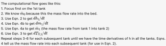
So the equations we're solving:casualguitar said:Besides this no further questions I am good to proceed. I'll write out the up to date model equations with the relevant substitutions now
The gas phase mole balance:
##m_{m,j}\frac{\partial y_{i,j}}{\partial t} = \dot{m}_{j-1}(y_{j-1} - y_j) - \dot{M}_{i,j}''A_{S,j} + y_{i,j}\sum_{j=1}^{n_c}\dot{M}_j^"A_S##
The gas phase heat balance:
##m_{m,j}c_{p,j}\frac{\partial T_{g,j}}{\partial t} = \dot{m}_{j-1}c_{p,j-1}(T_{j-1} - T_j) - q_{g,I,j}A_{S,j}##
Bed heat balance:
##M_{s,j}C_{p,s,j}\frac{\partial T_{b,j}}{dt}=q_{I,b,j}A_{S,j}##
Solid phase mass balance:
##A_C\Delta z\frac{\partial M_{i,j}}{\partial t} ={\dot{M}_{i,j}^"A_{S,j}}##
Variation of gas phase mass holdup w.r.t. time:
##\frac{\partial m_j}{\partial t} = \dot{m}_{j-1} - \dot{m}_j -\sum_{i=1}^{n_c}{\dot{M}_{i,j}^"A_{S,j}}##
##\frac{\partial m_j}{\partial t}=-\frac{\rho_{m,j}}{T_j}A_C\Delta z\frac{\partial T_{g,j}}{\partial t}##
Mass flow out of a tank:
##\dot{m}_j=\dot{m}_{j-1}+\frac{\rho_{m,j}}{T}A_C\Delta z\frac{\partial T}{\partial t}-\sum_{i=1}^{n_c}{\dot{M}_{i,j}^"A_{S,j}}##
Where:
##A_s = A_C\Delta za_s##
##M_s = \rho_s(1-\epsilon_g)A\Delta z##
##m_j=\rho_jA_C\epsilon \Delta x=\rho_j(V/n)##
##\dot{m_j}=\phi_{x+\Delta x/2}A_C\epsilon##
##A_{S,j}=A/n## where n is the number of tanks
##M_{S,j}=M/n##
Do these equations look ok? In your view are they in a final 'solvable' form?