casualguitar said:
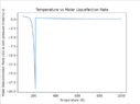
I haven't solved this yet, but I did find something odd. Solve_ivp offers a number of integrators (LSODA, Radau, RK45, RK23, DOP853, BDF). I tried a few and they all seem to return very different results. Actually all of them show the gas temperature reaching temperatures that are not present in the system at all which indicates I'm doing something wrong anyway, but regardless I didn't expect the output from each integrator do vary this much
For reference, these are the initial, boundary, and constant values I'm using. Anything stand out here to you as being a value that is outside its typical range?
n = 5 #number of tanks
rho0CO2 = 1.1 #initial density of CO2 in bed (mol/m3)
rho0H2O = 1.1 #initial density of h2o in bed (mol/m3)
y0CO2 = 0 #initial gas phase mole fraction of CO2 in bed (mol/mol)
y0H2O = 0 #initial gas phase mole fraction of h2o in bed (mol/mol)
M0CO2 = 0.0 #initial solid CO2 moles deposited on bed (mol/m2)
M0H2O = 0.0 #initial solid h2o moles deposited on bed (mol/m2)
Tg0 = 150 #initial gas temperature (K)
Tb0 = 150 #initial bed temperature (K)
A_C = 0.005 #cross sectional area (m2)
A_s = 267 #specific surface area of solid (m2/m3)
h_vap_h2o = 40650 (J/mol)
v_desublimation_co2 = 26000 (J/mol)
k_s = 18 #solid heat capacity (W/m.K)
dz = 0.01
U_b = 100 #bed heat transfer coefficient (W/m2.K)
U_g = 200 #gas phase heat transfer coefficient (W/m2.K)
cp_CO2 = 45 #co2 heat capacity (J/mol.K)
cp_H2O = 45 #h2o heat capacity (J/mol.K)
ki_co2 = 8 #co2 mass transfer coefficient (mol/m2.s)
ki_h2o = 16 #h2o Mass Transfer coefficient (mol/m2.s)
m_co2 = rho0CO2*dz*A_C (value of 5*10^-5)
m_h2o = rho0H2O*dz*A_C (value of 5*10^-5)
M_al = 72.2 (mol/tank) (about 7kg/tank)
#Boundary conditions
mol_in = 0.5 #mol/s
y_co2_in = 0.1 #mol/mol
y_h2o_in = 0.01 #mol/mol
T_in = 220 #K