a1titude
- 5
- 1
- Homework Statement
- It's not a homework. I just saw the resultant equation to find that it's strange.
- Relevant Equations
- $$\mathbf{B} = \mathbf{\nabla} \times \mathbf{A} = - \frac {\mu_0 m_0 \omega^2} {4 \pi c^2} \left( \frac {\sin \theta} {r} \right) \cos [\omega (t - r/c)] \hat{\mathbf{\theta}}$$
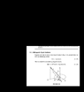
In 11.1.3 of Griffith's "Introduction to Electrodynamics 4Ed" appears magnetic dipole radiation, which results in the equation above. According to the resultant equation, there is no magnetic field in the axis of the wire loop because theta=0. However, I think the magnetic flux density is at maximum value there although its time-varying due to the alternating current. What am I missing now? Thanks for your concerns in advance.