Modelling of two phase flow in packed bed using conservation equations

[casualguitar]

TL;DR Summary

How can the conservation/Navier Stokes equations (mass, momentum,energy) be modified to model two phase flow in a porous media?

Previously, I have seen the derivation of the energy conservation equations for simulation of single phase flow in a porous media (a packed bed). These are the energy equations for the solid and fluid respectively:

I understand the derivation, however, these equations will only work when the fluid flow is single phase. I would like to derive this equation (and likely the mass/momentum equations if necessary), for two phase fluid flow i.e. with a phase change

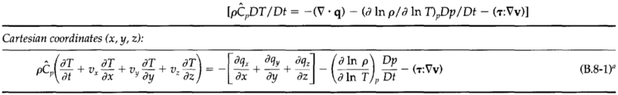
The mass, momentum, and energy conservation equations:

The goal here is to model the phase change of the fluid as it flows through the porous bed.

Requirements here are to model the temperature of the solid and fluid over time, and to track the phase fronts over time. Inside the phase change segment of the bed I would like to track the quality. I believe the solid energy conservation equation is not affected by the phase change, and we do not need mass/momentum conservation for the solid as it is static.

So this leaves a mass,momentum, and energy balance for the two phase fluid

I have set up a code base that allows calculation of almost any property for a pure fluid or mixture that would be required for this model. So essentially the derivation of the conservation equations are all that are remaining to model this system.

So to the question - how can I get started with deriving mass/momentum/energy (MME) equations that track the goal parameters? Is this a trivial change to the equations above?

Side note - I am also including this energy conservation equation that was previously flagged as being useful in solving this problem:

 

[Chestermiller]

This is a rather complicated problem, and attacking it will require good modeling strategy. The first principle of good modeling is to start simple and gradually build in complexity until you have a model that you are comfortable with. So starting with the most general mass, momentum, and energy balance equations that you have shown above and then trying to apply them to your situation is the opposite of what you should be doing. The first pair of equations you presented is much closer to where you should be heading.

What is needed are some preliminary calculations using a very simple model (or an array of simple models) to get your feet wet and get the "lay of the land." Also, it would quickly give you some results under your belt.

Do you have an idea of a starting design for this system, such as overall diameter, packing type, void fraction, length, bed orientation (vertical or horizontal), flow direction, etc? What is the gas/liquid, inlet fluid temperature, initial bed temperature, initial temperature and phase of fluid within bed, etc?

Let's brainstorm some preliminary models to get us started.

1. Two phase flow of vapor and liquid in a bed is going to be pretty complicated, particularly if the pressure is changing and the residence time is large. Let's model what the isothermal behavior of the fluid would be (a) if it were all liquid and (b) if it were all gas. This would give us an idea of the residence time and the possible pressure variations in the bed. This is all designed to give us a handle on the relevance of the fluid flow to this system.

2. Consider a case in which the pressure of the fluid is constant and there is a huge amount of axial dispersion in the fluid, so that that the fluid is all at the same temperature within the bed, and the exit temperature is the same as the fluid temperature within the bed. This is a so-called lumped parameter continuous stirred tank model. Under these circumstances, the bed temperature would also be uniform at any time. Assume first no phase change, and determine the fluid and bed temperatures as functions of time. Then solve it for a mixture of liquid and gas exiting.

Your turn to brainstorm some simplified models for this list. Also, let's see your formulation for the 2nd item on my list (at least for the no-phase-change case). If you have trouble with this, I will help.

 

[Chestermiller]

Once you set up the 2nd model I proposed, you will see how to modify the first fluid equation in your original post to include phase change.

 

[casualguitar]

Hi Chet!

Again much appreciated for your help on this. It's great to have someone to discuss this with. Apologies in advance for the slightly verbose response.

What is needed are some preliminary calculations using a very simple model (or an array of simple models) to get your feet wet and get the "lay of the land."

Ok great. You're right this is exactly the opposite of what I was planning to do. The idea of starting simple and gradually building the model does sound like a better approach. And yes it would also provide a map of results, rather than just having one final model with nothing to compare with.

Do you have an idea of a starting design for this system, such as overall diameter, packing type, void fraction, length, bed orientation (vertical or horizontal), flow direction, etc? What is the gas/liquid, inlet fluid temperature, initial bed temperature, initial temperature and phase of fluid within bed, etc?

Yes, I know all of these values actually. They will be variables in the model but I'll provide all values here to give a mental image of the system. The packed bed is intended to be a lab scale cryogenic energy storage system.

Diameter: 10cm approx
Packing type: random
Void fraction: about 0.3 (I don't have this number on hand). I should add here that the bed is static
Length: 2.8m approx
Bed Orientation: Vertical
Gas/Liquid: Air (O2/N2 mixture)
Flow Direction (there are two configurations here):
1) The bed is at ambient temperature and liquid air flows from the bottom up through the bed, vaporising and cooling the bed. The gas flows out through the top
2) Ambient temperature air flows down through a cold packed bed, liquefying the gas and warming the bed. The liquid flows out through the bottom
Initial Temperatures:
Configuration 1) Liquid air at approx 80K and a packed bed temperature of about 290K
Configuration 2) Ambient air at approx 290K and a packed bed at 80K

Initial thoughts on your two models:
1.
Pressure variation: Up until now I've assumed constant pressure, and any model I've seen has done the same. However in a system like this its possible that the pressure drop will be significant so I'll aim to have it in the final models down the line.
Residence time: I haven't thought about the residence time here. I initially assumed I would just any inlet flow value, however this seems to be incorrect. The fluid will surely need a given amount of time to liquefy/regasify, and maybe the flow rate should be set such that it gives the liquid/gas enough time to change phase
Modelling the residence time of a fluid/gas: Would this just be a calculation to find the pore velocity of the liquid/gas? Then the residence time would simply be Length/Pore velocity
Pressure Drop: I think I can do a simple calculation with the Ergun equation here to get an approx idea

2.
Ok to confirm I understand this correctly - the effect of very high axial dispersion is that at any time the bed will be the same temperature throughout. The fluid is also at the same temperature throughout, meaning that it must enter at temperature T0 and immediately change to temperature T1. Is the bed necessarily at temperature T1 also? I will need to do some reading on lumped parameter models, but I think the idea here is to take weighted average values of any model parameter (cp, density, etc) at any point?

Your turn to brainstorm some simplified models for this list. Also, let's see your formulation for the 2nd item on my list (at least for the no-phase-change case).

Ok I'm going to make my attempt at model 2 tonight/tomorrow. It seems simplification of the conservation equations is the way to go there. Is this a fair approach? Also, I see your second reply to this post was posted as I am writing this. I will reply to this separately. Thank you

 

[casualguitar]

Once you set up the 2nd model I proposed, you will see how to modify the first fluid equation in your original post to include phase change.

Oh Interesting!

Actually I should add, I am able to solve PDEs numerically and have done so for some simple models I found in various papers.

As mentioned I also wrote a library that can calculate any mixture or pure fluid property for gas/liquid phase (cp,rho etc). These properties are functions of temperature and pressure, so this will allow (slightly easier) implementation of the pressure variation model I would imagine

 

[anorlunda]

What ratios of liquid/gas are you considering? As the value of the ratio gets smaller, separation of the phases becomes important.

 

[casualguitar]

What ratios of liquid/gas are you considering? As the value of the ratio gets smaller, separation of the phases becomes important.

Hi and thank you for your response. I'm not sure I fully understand your question.

The inlet to the bed will always be either a gas or a liquid, never a mixture of the two. Inside the bed, the phase change will occur over a certain 'distance' inside the packed bed (gas to liquid, or liquid to gas), and the outlet will also ideally be single phase.

Does this answer your question? If it doesn't I can clarify any further questions on the design. Also, if you see my response to Chet Miller, I describe the system at a high level

 

[anorlunda]

The inlet to the bed will always be either a gas or a liquid, never a mixture of the two.

Sorry, I misread the question.

 

[casualguitar]

Sorry, I misread the question.

No bother at all and thanks for your response. I'm currently working on model 2 as proposed by Chet above. I am happy to discuss the model with you also. I should have an attempt at model 2 complete tomorrow morning (EU time here)

 

[Chestermiller]

Hi Chet!

Initial thoughts on your two models:
1.
Pressure variation: Up until now I've assumed constant pressure, and any model I've seen has done the same. However in a system like this its possible that the pressure drop will be significant so I'll aim to have it in the final models down the line.
Residence time: I haven't thought about the residence time here. I initially assumed I would just any inlet flow value, however this seems to be incorrect. The fluid will surely need a given amount of time to liquefy/regasify, and maybe the flow rate should be set such that it gives the liquid/gas enough time to change phase
Modelling the residence time of a fluid/gas: Would this just be a calculation to find the pore velocity of the liquid/gas? Then the residence time would simply be Length/Pore velocity

Yes.

Pressure Drop: I think I can do a simple calculation with the Ergun equation here to get an approx idea

Yes, this is what I had in mind.

2.
Ok to confirm I understand this correctly - the effect of very high axial dispersion is that at any time the bed will be the same temperature throughout. The fluid is also at the same temperature throughout, meaning that it must enter at temperature T0 and immediately change to temperature T1. Is the bed necessarily at temperature T1 also? I will need to do some reading on lumped parameter models, but I think the idea here is to take weighted average values of any model parameter (cp, density, etc) at any point?

Not exactly. The bed and the fluid (gas) in the bed start out at T1 while fluid (gas) is introduced into the bed at T0. So the temperature in the lumped parameter tank will start out at T1 and rise gradually to T0. There is a heat transfer coefficient between the bed and the gas in the bed. So the dependent variables will be the gas temperature and the bed temperature, and, in this simple model, they will be functions only of time.

 

[casualguitar]

Not exactly. The bed and the fluid (gas) in the bed start out at T1 while fluid (gas) is introduced into the bed at T0. So the temperature in the lumped parameter tank will start out at T1 and rise gradually to T0. There is a heat transfer coefficient between the bed and the gas in the bed. So the dependent variables will be the gas temperature and the bed temperature, and, in this simple model, they will be functions only of time.

Ok great. It seems we will only need the energy conservation equation here then for both the fluid and solid separately, not the mass/momentum equations. Is this correct?

So taking the energy conservation equation:

Assumptions:
1) No temperature variation along the bed in any direction for both the fluid and solid (dT/dx,dT/dy,dT/dz) will all be zero)
2) No pressure variation (Dp/Dt = 0)
3) The velocity gradient is small enough such that shear stresses will be zero (shear stress term will be zero)
4) We're dealing with a single phase

Point of confusion:
I'm going to say that q here is due to only convection, not the sum of convection and conduction. The reason I'm confused here is because the the temperature in the bed is constant. So this might mean there is no conduction between solid particles. Is this correct?

So for those reasons, I think the answer to model 2 is the same as the original equations I posted, minus the dTf/dx fluid term, the conduction terms in both equations, and the losses to the environment term. I'm going to write the equations out using LaTex (I haven't done this before so I guess it'll take a few attempts to get right):

$$\epsilon\ * \rho_{f} *C_{pf}*dT_{f}/dt = h_{fp}*a_{s}*(Ts-Tf)$$
$$(1-\epsilon) * \rho_{s} *C_{ps}*dT_{s}/dt = h_{fs}*a_{s}*(Tf-Ts)$$

These equations say the following to me:
LHS: The temperature of the fluid/solid will change over time
RHS: The temperature change is driven by convection (the difference between Tf and Ts)
Note: f and s subscripts are fluid and solid

Is this the right direction? I will edit this if I see any corrections!

I'm now going to look into how to adapt this for the phase change case. My initial thought is that it seems that it might be possible to have an 'if statement' of sorts, where we check the boiling point of the fluid. For T>Tsat we use the gas parameters, and for T<Tsat we use liquid parameters. This could avoid the need for a phase change term. However obviously it tells us nothing about the phase change itself.

I'm going to think about the addition of a phase change term now.

 

[Chestermiller]

For the lumped parameter model I described, in the case of no phase change, the overall mass balance on the gas is $$\frac{dm}{dt}=\dot{m}_{in}-\dot{m}_{out}$$and the enthalpy balance on the gas is $$\frac{d(mh)}{dt}=\dot{m}_{in}h_{in}-\dot{m}_{out}h-UA(T-T_S)$$where m is the mass of fluid in the bed at any time $\left(m=\frac{pM}{RT}V\right)$, $\dot{m}_{in}$ is the mass flow rate into the bed, $\dot{m}_{out}$ is the mass flow rate of gas out of the bed, U is the heat transfer coefficient between the gas and the solid bed, V is the total pore volume, and A is the heat transfer area between the gas and solid bed. Note that, in this crude lumped parameter model, all the gas is well mixed, so the exit enthalpy is equal to the uniform gas enthalpy in the bed.

Combining these two equations yields:
$$m\frac{dh}{dt}=\dot{m}_{in}(h_{in}-h)-UA(T-T_S)$$Substituting for the enthalpy $dh=C_PdT$, we then have: $$mC_p\frac{dT}{dt}=\dot{m}_{in}C_p(T_{in}-T)-UA(T-T_S)$$
For the solid bed, the corresponding heat balance is $$MC_S\frac{dT_S}{dt}=UA(T-T_S)$$
So, for this very crude lumped parameter model, we have two simultaneous ordinary differential equation in two unknowns for the gas temperature T and the solid bed temperature $T_S$. Note that this simple formulation accounts for the changes in gas holdup within the bed as a result of temperature induced density changes.

If it were me, I would run some calculations using this crude model to see what it predicted.

Extending this model to cases in which there is vapor condensation would be the next step. How do you think the equations would change in a region where vapor condensation is occurring at constant temperature and pressure.

 

[casualguitar]

Combining these two equations yields:
$$m\frac{dh}{dt}=\dot{m}_{in}(h_{in}-h)-UA(T-T_S)$$Substituting for the enthalpy $dh=C_PdT$, we then have: $$mC_p\frac{dT}{dt}=\dot{m}_{in}C_p(T_{in}-T)-UA(T-T_S)$$
For the solid bed, the corresponding heat balance is $$MC_S\frac{dT_S}{dt}=UA(T-T_S)$$
So, for this very crude lumped parameter model, we have two simultaneous ordinary differential equation in two unknowns for the gas temperature T and the solid bed temperature $T_S$. Note that this simple formulation accounts for the changes in gas holdup within the bed as a result of temperature induced density changes.

If it were me, I would run some calculations using this crude model to see what it predicted.

Extending this model to cases in which there is vapor condensation would be the next step. How do you think the equations would change in a region where vapor condensation is occurring at constant temperature and pressure.

Wow ok I was way off. I fully understand how you got the final solid/heat balances though. Again thank you for the comprehensive responses.

I'll put together a simulation for this model in Python.

Extending this model to cases in which there is vapor condensation would be the next step. How do you think the equations would change in a region where vapor condensation is occurring at constant temperature and pressure.

Ok so for the vapour condensation model, as we previously discussed, the solid heat balance stays the same. Hmm so to the fluid heat balance (I'll try to follow the logic you followed):

One point of confusion first:
Before I attempt the heat balance, can I ask - should I expect I will have two (or even three maybe) heat balances for the fluid? As follows:
Heat Balance 1: Specifically for the phase change zone and will include a phase change term with the heat of condensation
Heat Balance 2: For the single phase gas zone (before condensation)
Heat Balance 3: For the single phase liquid zone (after condensation)

Or does there exist a single heat balance equation that can model all three zones?

Reasoning for more than one heat balance for the fluid:
I'm thinking this is the case because I'm not sure how I could get the phase change term to be equal to zero for the regions outside the phase change region. I could possible imagine a $$\frac{dX}{dt}$$ derivative representing the phase change (where X is the liquid fraction). This term would need to be zero when the phase change is not happening. I could possible produce this derivative term from the mixture enthalpy equation:
$$h_{mix} = h_{l} * X + h_{g} * (1-X)$$

Are the above guesses correct? (I'd like to give this a proper attempt before any solution from you!). Thank you

 

[Chestermiller]

Wow ok I was way off. I fully understand how you got the final solid/heat balances though. Again thank you for the comprehensive responses.

I'll put together a simulation for this model in Python.
Ok so for the vapour condensation model, as we previously discussed, the solid heat balance stays the same. Hmm so to the fluid heat balance (I'll try to follow the logic you followed):

One point of confusion first:
Before I attempt the heat balance, can I ask - should I expect I will have two (or even three maybe) heat balances for the fluid? As follows:
Heat Balance 1: Specifically for the phase change zone and will include a phase change term with the heat of condensation
Heat Balance 2: For the single phase gas zone (before condensation)
Heat Balance 3: For the single phase liquid zone (after condensation)

Or does there exist a single heat balance equation that can model all three zones?

Reasoning for more than one heat balance for the fluid:
I'm thinking this is the case because I'm not sure how I could get the phase change term to be equal to zero for the regions outside the phase change region. I could possible imagine a $$\frac{dX}{dt}$$ derivative representing the phase change (where X is the liquid fraction). This term would need to be zero when the phase change is not happening. I could possible produce this derivative term from the mixture enthalpy equation:
$$h_{mix} = h_{l} * X + h_{g} * (1-X)$$

Are the above guesses correct? (I'd like to give this a proper attempt before any solution from you!). Thank you

Yes. This is basically all correct. The starting balance equations all still apply, but the equations for the enthalpy per unit mass and the holdup m of fluid will be more general:

If $T_R$ is a reference temperature for zero enthalpy of liquid and $T_{sat}$ is the saturation temperature at the bed pressure, then

$h=C_{PL}(T-T_R)$ for $T\leq T_{sat}$

$h=C_{PL}(T_{sat}-T_R)+\Delta h_{vap}(1-X)$ for $T=T_{sat}$ and $0 \leq X \leq1$

$h=C_{PL}(T_{sat}-T_R)+\Delta h_{vap}+C_{PV}(T-T_{sat})$ for $T \geq T_{sat}$

and, for the mass holdup in the column, if $v_L$ is the specific volume of the liquid, we have

$m=\frac{V}{v_L}$ for $T\leq T_{sat}$

$m=\frac{V}{v_lX+\frac{RT_{sat}}{PM}(1-X)}$ for $T=T_{sat}$ and $0 \leq X \leq1$

$m=\frac{PM}{RT}V$ for $T \geq T_{sat}$

I hope this makes sense

 

[Chestermiller]

Based on this simple model, it is now clear to me how to set up the numerical solution to the necessarily modified version of the original heat balance in your first post. But, before we discuss this, I'd be interested in seeing your results for the simplified model calculations. I'd like to see you get some experience with this first.

 

[casualguitar]

Based on this simple model, it is now clear to me how to set up the numerical solution to the necessarily modified version of the original heat balance in your first post. But, before we discuss this, I'd be interested in seeing your results for the simplified model calculations. I'd like to see you get some experience with this first.

Hi Chet, I just finished reading your comment on the phase change model. This mostly makes sense to me. Yes I can implement the no phase change model before we continue (not sure just yet on the phase change one). I do have some questions to clear up first though.

So we've got the fluid and solid heat balances from you above:
$$mC_p\frac{dT}{dt}=\dot{m}_{in}C_p(T_{in}-T)-UA(T-T_S)$$
$$MC_S\frac{dT_S}{dt}=UA(T-T_S)$$

We don't have any spatial derivatives, so we just need to discretise the time domain here (say increments of 1 second for example). We can then write the derivatives in the fluid/solid heat balances in numerical form (forward difference):
$$\frac{T^{t+1}_f - T^{t}_f}{\delta T}$$
$$\frac{T^{t+1}_s - T^{t}_s}{\delta T}$$

Then we can solve for $T^{t+1}_f$ and $T^{t+1}_s$ as we have values for all of the other parameters

Now, we need to update the values of $T$ (or $T_{f}$ as I've called it) and $T_{s}$, increment the time value, and repeat until $t$ = the set point value.

The values $m, C_{pf}$ and $C_{ps}$ should be updated each loop also. I can do this actually for the fluid (I don't have Cp correlations for the solid so I'll leave this constant)

The U value I will leave as a global variable (I could just adjust this freely for the purpose of this model, rather than finding correlations).

Finally, the A value will be the total surface area of the solid.

$$V_{totalsolids} = V*\epsilon$$
$$V_{particle} = \pi*\frac{d^2}{4}$$

From this I can find the number of particles and the total surface area, A

Is the above approach suitable? If so I can implement this in Python

 

[Chestermiller]

Hi Chet, I just finished reading your comment on the phase change model. This mostly makes sense to me. Yes I can implement the no phase change model before we continue (not sure just yet on the phase change one). I do have some questions to clear up first though.

So we've got the fluid and solid heat balances from you above:
$$mC_p\frac{dT}{dt}=\dot{m}_{in}C_p(T_{in}-T)-UA(T-T_S)$$
$$MC_S\frac{dT_S}{dt}=UA(T-T_S)$$

We don't have any spatial derivatives, so we just need to discretise the time domain here (say increments of 1 second for example). We can then write the derivatives in the fluid/solid heat balances in numerical form (forward difference):
$$\frac{T^{t+1}_f - T^{t}_f}{\delta T}$$
$$\frac{T^{t+1}_s - T^{t}_s}{\delta T}$$

Then we can solve for $T^{t+1}_f$ and $T^{t+1}_s$ as we have values for all of the other parameters

Now, we need to update the values of $T$ (or $T_{f}$ as I've called it) and $T_{s}$, increment the time value, and repeat until $t$ = the set point value.

The values $m, C_{pf}$ and $C_{ps}$ should be updated each loop also. I can do this actually for the fluid (I don't have Cp correlations for the solid so I'll leave this constant)

The U value I will leave as a global variable (I could just adjust this freely for the purpose of this model, rather than finding correlations).

Finally, the A value will be the total surface area of the solid.

$$V_{totalsolids} = V*\epsilon$$
$$V_{particle} = \pi*\frac{d^2}{4}$$

From this I can find the number of particles and the total surface area, A

Is the above approach suitable? If so I can implement this in Python

Regarding the heat capacities, do you really want to consider these temperature-dependent? At least for this crude model, I would treat them as constants.

Do you not have available to you an automatic ODE implicit integrator like the GEAR package on the IMSL library or DASSL (available for free online)? Of course, these are FORTRAN programs. Is there no such software available with PYTHON? It would make life so much easier for you, since these packages have automatic time step size control, automatic order control, and automatic accuracy control, and all you need to do is provide coding for calculating the time derivatives.

If you are going to integrate these equations manually, I strongly recommend going fully implicit. You are certainly going to have to do this (for stability control) when you solve the actual PDEs for the time- and spatial model.

 

[casualguitar]

Regarding the heat capacities, do you really want to consider these temperature-dependent? At least for this crude model, I would treat them as constants.

Will do. Its fairly straightforward for me to treat them as variable using the code I wrote to do this. I'll treat them as constant in this model.

Do you not have available to you an automatic ODE implicit integrator like the GEAR package on the IMSL library or DASSL (available for free online)? Of course, these are FORTRAN programs. Is there no such software available with PYTHON? It would make life so much easier for you, since these packages have automatic time step size control, automatic order control, and automatic accuracy control, and all you need to do is provide coding for calculating the time derivatives.

Hmm I hadn't thought about using something something like this. This would be a package that could solve both single ODEs and systems of PDEs I guess? Ok sounds good I'll go with this approach as it will be even more useful as the model develops as you said

If you are going to integrate these equations manually, I strongly recommend going fully implicit. You are certainly going to have to do this (for stability control) when you solve the actual PDEs for the time- and spatial model.

Yes I was thinking of using Crank Nicolson to solve future models and Neumann stability analysis to get stable time steps. However as you said if there are packages that do this for you then this is preferred.

Ok I'm going to first find a package that does this and then implement the model above. Will reply here with some high level results. Thank you

 

[Chestermiller]

I have some more ideas for you on this simple model.

For the case of constant heat capacity and no phase change,
1. Solve the equations analytically

2. Consider the limiting case where the fluid flow is so fast that it does not change temperature in passing through the bed

3. Consider the limiting case where the heat transfer coefficient between the bed and solid approaches zero, so that the incoming fluid just purges the initial temperature of the fluid in the bed (like a CSTR)

For the case of a. phase change, rather than having the heat of vaporization and the specific volume change occur at an exact temperature, distribute the changes linearly over a narrow temperature range of say 5 C. This would enable you eliminate the mass fraction X variation at the saturation temperature from the calculation and simply replace it by the temperature variation over the range.

 

[casualguitar]

I will be spending this morning on the previous model (had some TA work to do over the weekend). Thank you for these additional model examples, they're really useful.

For the case of constant heat capacity and no phase change,
1. Solve the equations analytically

I can do this (and compare the results with the numerical original model). I'm not so sure how to deal with the
$\int T \, dTs$ and the $\int Ts\, dT$ terms but I'll get to this

2. Consider the limiting case where the fluid flow is so fast that it does not change temperature in passing through the bed

Ok I can do this too. I'm very tempted here to say we won't need an energy balance to the fluid at all here. The bed energy balance will possibly remain the same also:
$$MC_S\frac{dT_S}{dt}=UA(T-T_S)$$
The only difference is that T is now constant, meaning that this should be easy to solve analytically. Is this problem similar to placing a solid into a 'very large' body of fluid?

3. Consider the limiting case where the heat transfer coefficient between the bed and solid approaches zero, so that the incoming fluid just purges the initial temperature of the fluid in the bed (like a CSTR)

Hmm. I'm struggling to see the difference between this model and model 2. So in model 2 the fluid definitely will not change temperature. If we assume that U is actually zero in model 3, then the fluid temperature will not change over time either (after the initial purge). I think this would mean that the heat balance to the bed is the same for model 2 and model 3

For the case of a. phase change, rather than having the heat of vaporization and the specific volume change occur at an exact temperature, distribute the changes linearly over a narrow temperature range of say 5 C.

Understood

This would enable you eliminate the mass fraction X variation at the saturation temperature from the calculation and simply replace it by the temperature variation over the range.

I think I understand. So from this equation:
$h=C_{PL}(T_{sat}-T_R)+\Delta h_{vap}(1-X)$ for $T=T_{sat}$ and $0 \leq X \leq1$

We would now want the $\Delta h_{vap}$ contribution to increase linearly over an interval $T1 \leq T \leq{T2}$.

So we could use a something like:
$h=C_{PL}(T_{sat}-T_R)+\Delta h_{vap}(\frac{T-T1}{T2-T1})$ for $T1 \leq T \leq{T2}$

Ok, I'm going to find an ODE/PDE solver for the original model and return here with some output

 

[Chestermiller]

I will be spending this morning on the previous model (had some TA work to do over the weekend). Thank you for these additional model examples, they're really useful.I can do this (and compare the results with the numerical original model). I'm not so sure how to deal with the
$\int T \, dTs$ and the $\int Ts\, dT$ terms but I'll get to this

Oops. Forgot about that. Try it using an average value of the fluid density over the temperature range. Then you would have two liner first order coupled ODEs. This could be used to compare with the numerical solution to validate it.

Ok I can do this too. I'm very tempted here to say we won't need an energy balance to the fluid at all here. The bed energy balance will possibly remain the same also:
$$MC_S\frac{dT_S}{dt}=UA(T-T_S)$$
The only difference is that T is now constant, meaning that this should be easy to solve analytically. Is this problem similar to placing a solid into a 'very large' body of fluid?

Yes. Exactly. This would give a good indicator of the approximate time constant for the actual problem.

Hmm. I'm struggling to see the difference between this model and model 2. So in model 2 the fluid definitely will not change temperature. If we assume that U is actually zero in model 3, then the fluid temperature will not change over time either (after the initial purge). I think this would mean that the heat balance to the bed is the same for model 2 and model 3

The equation here would be $$mC_p\frac{dT}{dt}=\dot{m}_{in}C_p(T_{in}-T)$$. This would give the approximate time constant for the fluid thermal response.

Understood

I think I understand. So from this equation:
$h=C_{PL}(T_{sat}-T_R)+\Delta h_{vap}(1-X)$ for $T=T_{sat}$ and $0 \leq X \leq1$

We would now want the $\Delta h_{vap}$ contribution to increase linearly over an interval $T1 \leq T \leq{T2}$.

So we could use a something like:
$h=C_{PL}(T_{sat}-T_R)+\Delta h_{vap}(\frac{T-T1}{T2-T1})$ for $T1 \leq T \leq{T2}$

Yes, exactly. Something like that. We can flesh it out later. We would do the same sort of thing for the specific volume of the mixture.

 

[casualguitar]

Oops. Forgot about that. Try it using an average value of the fluid density over the temperature range. Then you would have two liner first order coupled ODEs. This could be used to compare with the numerical solution to validate it.

Yes. Exactly. This would give a good indicator of the approximate time constant for the actual problem.

The equation here would be $$mC_p\frac{dT}{dt}=\dot{m}_{in}C_p(T_{in}-T)$$. This would give the approximate time constant for the fluid thermal response.

Yes, exactly. Something like that. We can flesh it out later. We would do the same sort of thing for the specific volume of the mixture.

Hi Chet, to our original two equation, single phase question - I've got a solution for this. I'll post the code plus the output below. The values of U and A and arbitrary so the solution has very little physical meaning but the main thing is that the solver seems to work! I'm going to save all of these models as they do all add value even if they're simplifications of the goal model.

The code:

The output (quite basic but it shows the solid and fluid temperature both trending towards the inlet fluid temperature):

 

[casualguitar]

Yes. Exactly. This would give a good indicator of the approximate time constant for the actual problem.

This would give the approximate time constant for the fluid thermal response.

Yes, exactly. Something like that. We can flesh it out later. We would do the same sort of thing for the specific volume of the mixture.

In regards to what the time constant for fluid thermal response is, I guess this is the 'rate' at which the temperature of the fluid/solid move towards the equilibrium temperature?

If the above solution looks good to you, I'll do both of these models now. I think I should do these before moving to the phase change model we discussed above.

 

[Chestermiller]

In regards to what the time constant for fluid thermal response is, I guess this is the 'rate' at which the temperature of the fluid/solid move towards the equilibrium temperature?

If the above solution looks good to you, I'll do both of these models now. I think I should do these before moving to the phase change model we discussed above.

What are the units of time on the figure?

 

[casualguitar]

What are the units of time on the figure?

The mass flow is kg/s so the time should be in seconds I believe. No?

 

[casualguitar]

What are the units of time on the figure?

Hi Chet, if you see no large errors in the model above I will continue on with the other discussed models (to get an approximation of the thermal response time)

 

[Chestermiller]

Hi Chet, if you see no large errors in the model above I will continue on with the other discussed models (to get an approximation of the thermal response time)

Why are there wiggles in the time response of the fluid?

 

[Chestermiller]

I will be spending this morning on the previous model (had some TA work to do over the weekend). Thank you for these additional model examples, they're really useful.I can do this (and compare the results with the numerical original model). I'm not so sure how to deal with the
$\int T \, dTs$ and the $\int Ts\, dT$ terms but I'll get to thisOk I can do this too. I'm very tempted here to say we won't need an energy balance to the fluid at all here. The bed energy balance will possibly remain the same also:
$$MC_S\frac{dT_S}{dt}=UA(T-T_S)$$
The only difference is that T is now constant, meaning that this should be easy to solve analytically. Is this problem similar to placing a solid into a 'very large' body of fluid?Hmm. I'm struggling to see the difference between this model and model 2. So in model 2 the fluid definitely will not change temperature. If we assume that U is actually zero in model 3, then the fluid temperature will not change over time either (after the initial purge). I think this would mean that the heat balance to the bed is the same for model 2 and model 3Understood

I think I understand. So from this equation:
$h=C_{PL}(T_{sat}-T_R)+\Delta h_{vap}(1-X)$ for $T=T_{sat}$ and $0 \leq X \leq1$

We would now want the $\Delta h_{vap}$ contribution to increase linearly over an interval $T1 \leq T \leq{T2}$.

So we could use a something like:
$h=C_{PL}(T_{sat}-T_R)+\Delta h_{vap}(\frac{T-T1}{T2-T1})$ for $T1 \leq T \leq{T2}$

I would use $$h=C_{PL}(T_1-T_R)+$$$$[C_{PL}(T_{sat}-T_1)+\Delta h_{vap}+C_{PV}(T_2-T_{sat})]\left(\frac{T-T1}{T2-T1}\right)$$

 

[casualguitar]

Why are there wiggles in the time response of the fluid?

I’m actually not sure, I’ll look into this. Its related to satisfying the stability criteria I think. I had this issue when I tried modelling the PDEs in my original question. When I approached the max stable time increment it started wiggling like that

 

[casualguitar]

I would use $$h=C_{PL}(T_1-T_R)+$$$$[C_{PL}(T_{sat}-T_1)+\Delta h_{vap}+C_{PV}(T_2-T_{sat})]\left(\frac{T-T1}{T2-T1}\right)$$

I’ll actually go straight into this phase change model this evening. Thank you and I’ll post results hopefully tomorrow

 

[Chestermiller]

Definitely. But it wouldn't happen if you went fully implicit (like backward Euler).

 

[casualguitar]

Definitely. But it wouldn't happen if you went fully implicit (like backward Euler).

Agreed. I checked and RK45 - or Runge-Kutta 4th and 5th order - the method used by solve_ivp in this case is explicit. The package offers implicit methods also (just involves changing the method = 'RK45' keyword).

I switched to LSODA, which is a wrapper from the FORTRAN solver ODEPACK, and the instability issue was fixed:

As I said, working on the phase change model this morning

 

[casualguitar]

I would use $$h=C_{PL}(T_1-T_R)+$$$$[C_{PL}(T_{sat}-T_1)+\Delta h_{vap}+C_{PV}(T_2-T_{sat})]\left(\frac{T-T1}{T2-T1}\right)$$

So given the heat balance to the fluid:
$m\frac{dh}{dt}=\dot{m}_{in}(h_{in}-h)-UA(T-T_S)$

And the enthalpy equation for the liquid:
$h=C_{PL}(T-T_R)$ for $T\leq T_{sat}$

Leaves us with this equation for the liquid phase:
$mC_{pL}\frac{dT}{dt}=\dot{m}_{in}C_p(T_{in}-T)-UA(T-T_S)$

I'm unsure about the phase change zone though (haven't tried the gas phase yet but it looks to be similar to this one). Heres my train of thought:

For $T1 \leq T \leq{T2}$, your equation is:

$h=C_{PL}(T_1-T_R)+$$[C_{PL}(T_{sat}-T_1)+\Delta h_{vap}+C_{PV}(T_2-T_{sat})]\left(\frac{T-T1}{T2-T1}\right)$

So we need to take the derivative of this term. The first term will be zero, as $T1$ and $T_R$ are constants. For me it seems to make sense to expand the fraction on the right to:

$m\frac{dh}{dt}=0+$$[C_{PL}(T_{sat}-T_1)+\Delta h_{vap}+C_{PV}(T_2-T_{sat})]\left(\frac{T}{T2-T1}\right)$$-$$[C_{PL}(T_{sat}-T_1)+\Delta h_{vap}+C_{PV}(T_2-T_{sat})]\left(\frac{T1}{T2-T1}\right)$

Now, the last term seems to be zero also as these terms are all constant (I know my definition of the derivative above is technically wrong as I'm still cancelling terms). This leaves us with:

$m\frac{dh}{dt}=$$[C_{PL}(T_{sat}-T_1)+\Delta h_{vap}+C_{PV}(T_2-T_{sat})]\left(\frac{T}{T2-T1}\right)$

If the above is correct, this gives us the final equation for $\frac{dh}{dt}$, I'm not sure how to go from this to a $\frac{dT}{dt}$ term though, as we can't just sub in $dh = C_{pL}\frac{dT}{dt}$ like before.

Is the above approach correct? If so, how could I go about getting a dT/dt term from the dh/dt term?

 

[Chestermiller]

So given the heat balance to the fluid:
$m\frac{dh}{dt}=\dot{m}_{in}(h_{in}-h)-UA(T-T_S)$

And the enthalpy equation for the liquid:
$h=C_{PL}(T-T_R)$ for $T\leq T_{sat}$

Leaves us with this equation for the liquid phase:
$mC_{pL}\frac{dT}{dt}=\dot{m}_{in}C_p(T_{in}-T)-UA(T-T_S)$

I'm unsure about the phase change zone though (haven't tried the gas phase yet but it looks to be similar to this one). Heres my train of thought:

For $T1 \leq T \leq{T2}$, your equation is:

$h=C_{PL}(T_1-T_R)+$$[C_{PL}(T_{sat}-T_1)+\Delta h_{vap}+C_{PV}(T_2-T_{sat})]\left(\frac{T-T1}{T2-T1}\right)$

So we need to take the derivative of this term. The first term will be zero, as $T1$ and $T_R$ are constants. For me it seems to make sense to expand the fraction on the right to:

$m\frac{dh}{dt}=0+$$[C_{PL}(T_{sat}-T_1)+\Delta h_{vap}+C_{PV}(T_2-T_{sat})]\left(\frac{T}{T2-T1}\right)$$-$$[C_{PL}(T_{sat}-T_1)+\Delta h_{vap}+C_{PV}(T_2-T_{sat})]\left(\frac{T1}{T2-T1}\right)$

Now, the last term seems to be zero also as these terms are all constant (I know my definition of the derivative above is technically wrong as I'm still cancelling terms). This leaves us with:

$m\frac{dh}{dt}=$$[C_{PL}(T_{sat}-T_1)+\Delta h_{vap}+C_{PV}(T_2-T_{sat})]\left(\frac{T}{T2-T1}\right)$

If the above is correct, this gives us the final equation for $\frac{dh}{dt}$, I'm not sure how to go from this to a $\frac{dT}{dt}$ term though, as we can't just sub in $dh = C_{pL}\frac{dT}{dt}$ like before.

Is the above approach correct? If so, how could I go about getting a dT/dt term from the dh/dt term?

Between T1 and T2, it's just $$\frac{dh}{dt}=C^*\frac{dT}{dt}$$where $$C^*=\frac{[C_{PL}(T_{sat}-T_1)+\Delta h_{vap}+C_{PV}(T_2-T_{sat})]}{(T_2-T_1)}$$So, it's just a large constant heat capacity between T1 and T2.

What do you get for m in the three temperature regions?

 

[casualguitar]

Between T1 and T2, it's just $$\frac{dh}{dt}=C^*\frac{dT}{dt}$$where $$C^*=\frac{[C_{PL}(T_{sat}-T_1)+\Delta h_{vap}+C_{PV}(T_2-T_{sat})]}{(T_2-T_1)}$$So, it's just a large constant heat capacity between T1 and T2.

What do you get for m in the three temperature regions?

Ahh I see my apologies, yes what I did above is right except I forgot to replace $T$ with the derivative $\frac{dT}{dt}$ on the right. Should it not be (adding in m below the line. I guess you're leaving it out for me to fill it in):
$$C^*=\frac{[C_{PL}(T_{sat}-T_1)+\Delta h_{vap}+C_{PV}(T_2-T_{sat})]}{m(T_2-T_1)}$$

So m is constant outside the phase change zone. Inside the 'phase change' zone as you said its:
$$m=\frac{V}{v_lX+\frac{RT_{sat}}{PM}(1-X)}$$

I think we want the bottom line (average specific volume) to linearly increase from $v_l$ to $v_g$ over the interval $T1 \leq T \leq{T2}$, so we could just replace $1-X$ with $\frac{T-T1}{T2-T1}$, to give:

$$m=\frac{V}{v_l(1-\frac{T-T1}{T2-T1})+\frac{RT}{PM}(\frac{T-T1}{T2-T1})}$$

At $T=T1$ we are left with $v_l$ and at $T=T2$ we have $v_g$

How does this look?

 

[Chestermiller]

Ahh I see my apologies, yes what I did above is right except I forgot to replace $T$ with the derivative $\frac{dT}{dt}$ on the right. Should it not be (adding in m below the line. I guess you're leaving it out for me to fill it in):
$$C^*=\frac{[C_{PL}(T_{sat}-T_1)+\Delta h_{vap}+C_{PV}(T_2-T_{sat})]}{m(T_2-T_1)}$$

Not really. Between T1 and T2, we have $$m\frac{dh}{dt}=mC^*\frac{dT}{dt}=RHS$$where C* is as I wrote it in post #34. h is the enthalpy per unit mass.

So m is constant outside the phase change zone. Inside the 'phase change' zone as you said its:
$$m=\frac{V}{v_lX+\frac{RT_{sat}}{PM}(1-X)}$$

I think we want the bottom line (average specific volume) to linearly increase from $v_l$ to $v_g$ over the interval $T1 \leq T \leq{T2}$, so we could just replace $1-X$ with $\frac{T-T1}{T2-T1}$, to give:

$$m=\frac{V}{v_l(1-\frac{T-T1}{T2-T1})+\frac{RT}{PM}(\frac{T-T1}{T2-T1})}$$

For between T1 and T2, I get $$m=\frac{V}{\left[v_l+\left(\frac{RT_2}{PM}-v_l\right)\left(\frac{T-T_1}{T_2-T_1}\right)\right]}$$

 

[casualguitar]

Not really. Between T1 and T2, we have $mdhdt=mC∗dTdt=RHSwhere$ C* is as I wrote it in post #34. h is the enthalpy per unit mass.

Got it. I rewrote the derivative as above and it makes sense now

For between T1 and T2, I get: $$m=\frac{V}{\left[v_l+\left(\frac{RT_2}{PM}-v_l\right)\left(\frac{T-T_1}{T_2-T_1}\right)\right]}$$

Hmm interesting. Ok rearranging my equation, I get your one, except instead of $\frac{RT_2}{PM}$ I have $\frac{RT}{PM}$. Why do you use $T2$ instead of $T$ for the gas specific volume?

My guess is that you're saying the gas specific volume is a constant (doesn't vary with temperature). Also you're treating the liquid specific volume as a constant also. Could we not use T instead of T2 here if we wanted to treat the gas specific volume as temperature dependent? We would also need to treat $V_L$ as constant in that case I would guess

I'm going to start now on the code for this using your equations

 

[casualguitar]

Not really. Between T1 and T2, we have $$m\frac{dh}{dt}=mC^*\frac{dT}{dt}=RHS$$where C* is as I wrote it in post #34. h is the enthalpy per unit mass.

For between T1 and T2, I get $$m=\frac{V}{\left[v_l+\left(\frac{RT_2}{PM}-v_l\right)\left(\frac{T-T_1}{T_2-T_1}\right)\right]}$$

So summing up the last number of posts, this seems to be the current phase change model.

The general heat balance to the fluid is:
$$mC_p\frac{dT}{dt}=\dot{m}_{in}C_p(T_{in}-T)-UA(T-T_S)$$

Where $C_P$ is:

$C_{PL}$ for $T \leq T1$
$C_{PV}$ for $T \geq T2$
$C*$ for $T1 \leq T \leq{T2}$ where $(C^*=\frac{[C_{PL}(T_{sat}-T_1)+\Delta h_{vap}+C_{PV}(T_2-T_{sat})]}{(T_2-T_1)}$

and where $m$ is:

$\frac{V}{V_L}$ for $T \leq T1$
$\frac{PM}{RT_2}V$ for $T \geq T2$
$\frac{V}{\left[v_l+\left(\frac{RT_2}{PM}-v_l\right)\left(\frac{T-T_1}{T_2-T_1}\right)\right]}$ for $T1 \leq T \leq{T2}$

The general heat balance to the solid remains the same for each temperature range:
$$MC_S\frac{dT_S}{dt}=UA(T-T_S)$$

So essentially this model is two coupled differential equations that are solved for a range of times, where the values of $C_P$ and $m$ are chosen based on the temperature.

How does this look?

 

[Chestermiller]

Got it. I rewrote the derivative as above and it makes sense now

Hmm interesting. Ok rearranging my equation, I get your one, except instead of $\frac{RT_2}{PM}$ I have $\frac{RT}{PM}$. Why do you use $T2$ instead of $T$ for the gas specific volume?

In the interval between T1 and T2, I'm expressing the specific volume as a linear function of T, varying from $v_l$ at T1 to the gas specific volume at T2, namely $\frac{RT_2}{pM}$. The linear dependence on T is controlled by $\frac{T-T_1}{T_2-T_1}$

 

[casualguitar]

In the interval between T1 and T2, I'm expressing the specific volume as a linear function of T, varying from $v_l$ at T1 to the gas specific volume at T2, namely $\frac{RT_2}{pM}$. The linear dependence on T is controlled by $\frac{T-T_1}{T_2-T_1}$

Just letting you know I was sidetracked with some other project work for the last few days. I'm working on the post #38 now

 

[casualguitar]

In the interval between T1 and T2, I'm expressing the specific volume as a linear function of T, varying from $v_l$ at T1 to the gas specific volume at T2, namely $\frac{RT_2}{pM}$. The linear dependence on T is controlled by $\frac{T-T_1}{T_2-T_1}$

Hi Chet, phase change model code below with a graph of the fluid and solid temperatures over time. I could tweak the inputs until the graph looks nicer but in the interest of saving time I wont. Basically the code is exactly the same as the last model, except now we just take m and cp as variable rather than constant (as shown in the mass and cp functions).

So looking at the graph, initially the fluid temperature and the solid temperature jump towards one another, and then gradually both reduce to the gas inlet temperature. This happens slowly though, meaning that the mass flow in is small relative to the volume holdup. We also have the linear increase/decrease in temperature between T1 and T2 (shown by the straight line sections on the blue curve)

How does this look to you? What are your thoughts on adding in temperature variation along the direction of flow? Is this a reasonable development?

 

[Chestermiller]

Hi Chet, phase change model code below with a graph of the fluid and solid temperatures over time. I could tweak the inputs until the graph looks nicer but in the interest of saving time I wont. Basically the code is exactly the same as the last model, except now we just take m and cp as variable rather than constant (as shown in the mass and cp functions).

View attachment 292166
View attachment 292167
View attachment 292169
So looking at the graph, initially the fluid temperature and the solid temperature jump towards one another, and then gradually both reduce to the gas inlet temperature. This happens slowly though, meaning that the mass flow in is small relative to the volume holdup. We also have the linear increase/decrease in temperature between T1 and T2 (shown by the straight line sections on the blue curve)

How does this look to you? What are your thoughts on adding in temperature variation along the direction of flow? Is this a reasonable development?

This doesn't look anything like what I expected. I was expecting to see something like the previous graph. Wasn't the initial temperature of the bed supposed to be < 80 K, and the gas temperature supposed to be about 300 K? What did you use for T1 and T2, for the inlet gas temperature, and for the bed-filled-with-liquid temperature? Also, on the graph, please show times from 0 to 1000 s only.

 

[casualguitar]

This doesn't look anything like what I expected. I was expecting to see something like the previous graph. Wasn't the initial temperature of the bed supposed to be < 80 K, and the gas temperature supposed to be about 300 K? What did you use for T1 and T2, for the inlet gas temperature, and for the bed-filled-with-liquid temperature? Also, on the graph, please show times from 0 to 1000 s only.

Ah my apologies, the $80K/300K$ temperatures refer to the liquefaction of air model. I just chose water/steam for the model above to test this phase change model. I've switched it now so the initial temperature of the bed and fluid in the bed are both $80K$, and the gas entering is $300K$. I used $T1 = 100K$ and $T2 = 110K$ to approximate a boiling range. Range adjusted to $1000s$ also. I've also switched the input values (cp, vL, etc to reflect average air properties).

My apologies for the confusion there. What are your thoughts on adding in temperature variation along the direction of flow? Is this a reasonable development?

 

[Chestermiller]

Ah my apologies, the $80K/300K$ temperatures refer to the liquefaction of air model. I just chose water/steam for the model above to test this phase change model. I've switched it now so the initial temperature of the bed and fluid in the bed are both $80K$, and the gas entering is $300K$. I used $T1 = 100K$ and $T2 = 110K$ to approximate a boiling range. Range adjusted to $1000s$ also. I've also switched the input values (cp, vL, etc to reflect average air properties).
View attachment 292183
My apologies for the confusion there. What are your thoughts on adding in temperature variation along the direction of flow? Is this a reasonable development?

I assume you've run a range of test cases to put the model through its paces and get a feel for the quantitative effects of some of the parameters such as the heat transfer coefficient.

I'm hoping that you have developed an appreciation for the value of solving simple crude models of a system first before going to the more complicated versions. In this case, you have been able to develop a strategy for including the thermodynamics of the phase change in the calculations. Imagine having tried to do this with the full version of the model. You also have some results under your belt, so you already have a feel for the time scale of the behavior; the time for the system to be fully purged is going to be on the order of about 15 minutes. In my judgment, this has been of tremendous value. Please try to incorporate this kind of approach, in building from simple models to more complicated ones, as part of your routine strategy for the future.

We are going to need to have some discussions on expanding this to include the axial variation. I've been working on a finite difference scheme that I would be comfortable with for axial discretization; I'm close to finishing, and will document it for your consideration when I'm done. We also need to address dealing with numerical issues associated with advection/diffusion situations like this. Are you familiar with the concept of axial dispersion (over and above conduction ) in porous media and packed beds? Are you familiar with the "method of lines" for solving partial differential equations involving time and spatial position?

 

[casualguitar]

I assume you've run a range of test cases to put the model through its paces and get a feel for the quantitative effects of some of the parameters such as the heat transfer coefficient.

I'm hoping that you have developed an appreciation for the value of solving simple crude models of a system first before going to the more complicated versions. In this case, you have been able to develop a strategy for including the thermodynamics of the phase change in the calculations. Imagine having tried to do this with the full version of the model. You also have some results under your belt, so you already have a feel for the time scale of the behavior; the time for the system to be fully purged is going to be on the order of about 15 minutes. In my judgment, this has been of tremendous value. Please try to incorporate this kind of approach, in building from simple models to more complicated ones, as part of your routine strategy for the future.

Yes I've played with the input parameters to get an idea of how much of an effect it has on the output. I have got a more intuitive idea now as for how the system reacts to changes in input. Yes I would not have been able to do this with a full scale model, so really I suppose it can be faster to build simple models up gradually rather than go straight for the full version. I will incorporate this approach for future models!

We are going to need to have some discussions on expanding this to include the axial variation.

Great. I'm ready for this discussion now also

I've been working on a finite difference scheme that I would be comfortable with for axial discretization; I'm close to finishing, and will document it for your consideration when I'm done.

Thank you for this again, it is hugely appreciated. I won't ask too many questions yet but I thought we were avoiding manually implementing these FD schemes and instead using existing libraries to solve PDEs? I assume I'm misunderstanding what you mean by this

We also need to address dealing with numerical issues associated with advection/diffusion situations like this. Are you familiar with the concept of axial dispersion (over and above conduction ) in porous media and packed beds? Are you familiar with the "method of lines" for solving partial differential equations involving time and spatial position?

Not really. Axial dispersion refers to generally undesirable heat transfer both along the direction of flow and against the direction of flow I believe? For example over time the temperature gradient in a packed bed would reduce due to the temperature differences between the high and low temperature zones. I don't know why this would be different to conduction though. I assumed it would be a combination of conduction and convection.

I am not familiar with numerical issues associated with advection/diffusion, and no I'm not familiar with the method of lines either.

So in the meantime I will read up on the method of lines and axial dispersion and respond here with a new understanding

 

[Chestermiller]

To use the package codes to solve PDEs, you need to first discretize the equations spatially, but retain the time derivatives, which now become ordinary time derivatives. So you will be solving a set of coupled first order ordinary differential equations in time for the temperatures as the spatial grid points. This is called the method of lines. The package codes automatically solve these, and certain options guarantee stability of the time integration.

 

[casualguitar]

To use the package codes to solve PDEs, you need to first discretize the equations spatially, but retain the time derivatives

Understood. I did some reading on solving PDEs with the solve_ivp package I've used above and yes they generally said something similar to what you have said.

So you will be solving a set of coupled first order ordinary differential equations in time for the temperatures as the spatial grid points. This is called the method of lines.

I have seen solutions of PDEs similar to the ones I included in my original question that use methods like Crank Nicolson etc to solve for the temperature profiles at each time increment, where both the time and space domains are discretised. Why choose the method of lines approach over an approach like this?

 

[casualguitar]

To use the package codes to solve PDEs, you need to first discretize the equations spatially, but retain the time derivatives, which now become ordinary time derivatives. So you will be solving a set of coupled first order ordinary differential equations in time for the temperatures as the spatial grid points. This is called the method of lines. The package codes automatically solve these, and certain options guarantee stability of the time integration.

Hi Chet, just a quick update - I have now read up on the method of lines and have followed an example solution in MATLAB. To answer my own previous question regarding the use cases for the MOL, it seems the MOL would be chosen to take advantage of the methods and software that have been developed for numerically integrating ODEs

 

[Chestermiller]

You need to read up on axial heat dispersion in packed beds (over and above axial heat conduction). We need to discuss how to handle this.

 

[casualguitar]

You need to read up on axial heat dispersion in packed beds (over and above axial heat conduction). We need to discuss how to handle this.

Understood. I will read up on this now. Any aspects of porous media axial dispersion in particular? If not I will read up on how axial dispersion in packed beds is modeled. Thank you