Modelling of two phase flow in packed bed using conservation equations

[casualguitar]

Note finally, that, with no loss of generality, we can simplify further by taking the reference temperature for zero enthalpy of the liquid as Tsat, such that hsat,L=0 and hsat,V=Δhvaporization.

Got it, so just adding that in:

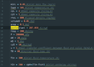
1. If $h\leq h_{sat,L}$, then
$$T=T_{sat}+h/C_{PL}$$
$$m=\rho_L V$$

2. If $h_{sat,L}\leq h \leq h_{sat,V}$ then
$$T=T_{sat}$$
$$m=\frac{V}{\left[\frac{1}{\rho_L}+\left(\frac{RT_{sat}}{PM}-\frac{1}{\rho_L}\right)\left(\frac{h}{\Delta h_{vap}}\right)\right]}$$

3. If $h_{sat,V}\leq h$ then
$$T=T_{sat}+(h-\Delta h_{vap})/C_{PV}$$
$$m=\frac{PM}{RT} V$$

We expect that the results of this calculation will match the results from the temperature-version, so it should provide a good validation of the model.

The post #38 model yes?

This method gets us out of the artificial approach of using T1 and T2, and is "exact" for the relations between enthalpy, temperature. and mass.

It does, I guess dealing with a mixture means that we should get an average value for $T_{sat}$ here (N2 boils at 77K, O2 boils at 90K) so maybe a Tsat of 73.5K is suitable here? The same for any other constant I could take the average of the N2 and O2 values.

I think I follow this model fully so, I will aim to implement this tomorrow morning!

 

[Chestermiller]

Got it, so just adding that in:

More like

1. If $h\leq 0$, then
$$T=T_{sat}+h/C_{PL}$$
$$m=\rho_L V$$

2. If $0\leq h \leq \Delta h_{vap}$ then
$$T=T_{sat}$$
$$m=\frac{V}{\left[\frac{1}{\rho_L}+\left(\frac{RT_{sat}}{PM}-\frac{1}{\rho_L}\right)\left(\frac{h}{\Delta h_{vap}}\right)\right]}$$

3. If $\Delta h_{vap}\leq h$ then
$$T=T_{sat}+(h-\Delta h_{vap})/C_{PV}$$
$$m=\frac{PM}{RT} V$$

The post #38 model yes?

Yes.

It does, I guess dealing with a mixture means that we should get an average value for $T_{sat}$ here (N2 boils at 77K, O2 boils at 90K) so maybe a Tsat of 73.5K is suitable here? The same for any other constant I could take the average of the N2 and O2 values.

Please use your best judgment for this. I guess at some point the model can be modified to more the precise VLE behavior. I think the 73.5 is a typo, and you meant 83.5, right?

 

[Chestermiller]

I think I can solve for the case with U = 0 analytically.

 

[casualguitar]

Working on the above model now I should have results for this in an hour or so. I'll change the inputs of the model we're comparing to so that they're close to equivalent. What would a U = 0 model show us? The effect of having zero heat transfer between fluid and solid?

 

[Chestermiller]

Working on the above model now I should have results for this in an hour or so. I'll change the inputs of the model we're comparing to so that they're close to equivalent. What would a U = 0 model show us? The effect of having zero heat transfer between fluid and solid?

It would tell us the effect of purging liquid initially at a low temperature from the lumped mixed tank with a vapor at a high temperature.

 

[casualguitar]

It would tell us the effect of purging liquid initially at a low temperature from the lumped mixed tank with a vapor at a high temperature.

So I made the above model, and ran it for ranges of input parameters etc. I've printed the output and I can see the expected increase of temperature to the saturation temperature, a (short) constant temperature zone, and then an increase up to the fluid inlet temperature. I've checked that the correct enthalpy/mass equations are being used for the right enthalpy ranges. I've also made this models inputs as close as possible to the old model inputs. This one produces results that are quite a bit different, in that the temperature of the fluid and gas increase at a much slower rate. I'm attaching the output to model 1 and 2, and also the code to the new model below. Note I plotted over 10000s as this was the time required to see a levelling out of the temperature curve in the new model. I'm assuming for now there is a bug in my code somewhere so I'll hopefully find it this evening!

New model:

Old model:

Enthalpy model code:

 

[Chestermiller]

I don’t see anything like a constant temperature zone in either plot. What were the parameter values you used, including the mass flow rate in, and the solid mass and heat capacity?

 

[casualguitar]

I don’t see anything like a constant temperature zone in either plot. What were the parameter values you used, including the mass flow rate in, and the solid mass and heat capacity?

There is a constant temperature zone in the new plot, however it’s very small (I think it spans only a few seconds). I’m away from my laptop currently so I will zoom in on this in the plot later this evening. In regards to mass flow in, solid mass and heat capacity, these are minL, mS and cpS in the first code image. I’ll also change these parameters this evening to get a longer constant temperature zone

 

[Chestermiller]

There is a constant temperature zone in the new plot, however it’s very small (I think it spans only a few seconds). I’m away from my laptop currently so I will zoom in on this in the plot later this evening. In regards to mass flow in, solid mass and heat capacity, these are minL, mS and cpS in the first code image. I’ll also change these parameters this evening to get a longer constant temperature zone

You omitted multiplying by the bed volume when you calculated the mass of fluid in the bed for pure vapor. This is an indication that you really need to spend some time testing and checking your code.

What are the units of the physical parameters in your code?

Heat transfer coefficeint
Heat transfer area
Heat capacity of bed
mass of bed

 

[casualguitar]

You omitted multiplying by the bed volume when you calculated the mass of fluid in the bed for pure vapor.

Thanks!

This is an indication that you really need to spend some time testing and checking your code.

Yes I agree completely. I did spend over an hour looking, however this is really a bug I should have been able to find if I'd spent some more time. I'll take more care to find these myself from now on

What are the units of the physical parameters in your code?

Units included in the comments here:

Updated graph below. Shows the constant temperature zone and levels out at the same rate:

I'm going to make a graph of this one over the previous model graph to see how well they actually overlay. However from visual inspection of the individual graphs they look ok

 

[Chestermiller]

It seems to me what is happening in this calculation is that the heat transfer resistance between the gas an the bed is very low (equivalent to very high heat transfer coefficient) so that the gas always comes very close to the bed temperature. Moreover, once the temperature rises above $T_{sat}$, there is all gas in the tank, and the thermal inertia of this gas is very low compared to the thermal inertia of the bed. So it can be neglected. So the rate at which the incoming gas gives up heat to the bed is $\dot{m}C_{PV}(T_{in}-T_S)$ and the heat balance on the bed in this range of temperatures simplifies to $$m_SC_{PS}\frac{dT_S}{dt}=\dot{m}C_{PV}(T_{in}-T_S)$$
This same result can be obtained by (a) eliminating the heat transfer term between the gas heat balance and solid heat balance, then (b) setting the instantaneous gas temperature in the bed equal to the bed temperature and then (c) neglecting the thermal inertia of the gas.

The characteristic time constant for the system in this range of temperatures is then $$\tau=\frac{m_SC_{PS}}{\dot{m}C_{PV}}$$What is the value that you calculate for this time constant for your model inputs?

 

[casualguitar]

What is the value that you calculate for this time constant for your model inputs?

Just adding the comparison graph here as mentioned before

Moreover, once the temperature rises above Tsat, there is all gas in the tank, and the thermal inertia of this gas is very low compared to the thermal inertia of the bed. So it can be neglected.

Understood

This same result can be obtained by (a) eliminating the heat transfer term between the gas heat balance and solid heat balance, then (b) setting the instantaneous gas temperature in the bed equal to the bed temperature and then (c) neglecting the thermal inertia of the gas.

Understood also.

The characteristic time constant for the system in this range of temperatures is then τ=mSCPSm˙CPVWhat is the value that you calculate for this time constant for your model inputs?

$M_S$ = 1, $C_{PS}$ = 10, $mass flow (kg/s) = 0.05$, $C_{PV}$ = 1, which returns the time constant:
$$\tau=200$$

I haven't looked into what a time constant of 200s means yet (quite late here). My initial sense is that it is very large. I will do this first thing tomorrow

I've also spotted an error in my previous model. The heat capacity of the solid is higher than any reasonable value for materials of its type (typical values are between 0.8 and 2). I'll rerun with a reasonable value tomorrow morning.

Looking at the time constant equation, a solid heat capacity of 1, for example, reduces the time constant to 20s which seems a lot more reasonable.

As I say I'll make these changes in the morning

 

[Chestermiller]

View attachment 292463
Just adding the comparison graph here as mentioned before

UnderstoodUnderstood also.
$M_S$ = 1, $C_{PS}$ = 10, $mass flow (kg/s) = 0.05$, $C_{PV}$ = 1, which returns the time constant:
$$\tau=200$$

I haven't looked into what a time constant of 200s means yet (quite late here). My initial sense is that it is very large. I will do this first thing tomorrow

I've also spotted an error in my previous model. The heat capacity of the solid is higher than any reasonable value for materials of its type (typical values are between 0.8 and 2). I'll rerun with a reasonable value tomorrow morning.

Looking at the time constant equation, a solid heat capacity of 1, for example, reduces the time constant to 20s which seems a lot more reasonable.

As I say I'll make these changes in the morning

Nice. Please make a semi-log plot of $T_{in}-T$ as a function of t, and let's see what you get.

I should also mention that the R in the equations I wrote is the universal gas constant, not the customized value for air. This has caused the masses of vapor you have used in the calculations to be a factor of 28 too high.

 

[casualguitar]

Nice. Please make a semi-log plot of $T_{in}-T$ as a function of t, and let's see what you get.

I should also mention that the R in the equations I wrote is the universal gas constant, not the customized value for air. This has caused the masses of vapor you have used in the calculations to be a factor of 28 too high.

Updating the overlay plot here with a solid heat capacity of $1.1 kJ/kg.K$. As expected the temperature levels off at a faster rate

I should also mention that the R in the equations I wrote is the universal gas constant, not the customized value for air.

Got it. So I should divide my value by the molecular weight, meaning that the new units for $R$ are $J/mol.K$?

Making the semi-log plot now

 

[casualguitar]

Nice. Please make a semi-log plot of $T_{in}-T$ as a function of t, and let's see what you get.

$T_{in} - T$ plot for the enthalpy model:

To be clear, what I did here was took the final temperature arrays for the fluid and solid, and then created two new arrays $(T_{in}-T_{fluid})$ and $(T_{in}-T_{solid})$ and plotted these versus $t$

 

[Chestermiller]

Updating the overlay plot here with a solid heat capacity of $1.1 kJ/kg.K$. As expected the temperature levels off at a faster rate
View attachment 292479Got it. So I should divide my value by the molecular weight, meaning that the new units for $R$ are $J/mol.K$?

Making the semi-log plot now

No. You multiply your value by 28 kg/(k-mole) to get $R=8314\ J/(k-mole\ K)$

 

[Chestermiller]

$T_{in} - T$ plot for the enthalpy model:
View attachment 292480
To be clear, what I did here was took the final temperature arrays for the fluid and solid, and then created two new arrays $(T_{in}-T_{fluid})$ and $(T_{in}-T_{solid})$ and plotted these versus $t$

Good. Now have your plotting software change the ordinate scale to logarithmic.

 

[casualguitar]

No. You multiply your value by 28 kg/(k-mole) to get $R=8314\ J/(k-mole\ K)$

Ok, new plot below with the updated R value. The effect of the updated R value is that the time taken to reach steady state is approximately cut in half:

Good. Now have your plotting software change the ordinate scale to logarithmic.

Both time and temperature axes to log scale?

 

[casualguitar]

Good. Now have your plotting software change the ordinate scale to logarithmic.

Here is the plot when both x and y are plotted in log scale:

What is the value of this plot? It shows us that at the later times (in the gas phase) the temperatures rises more rapidly towards the inlet gas temperature, meaning that (as you said) the thermal inertia of the gas is very low compared to the thermal inertia of the bed?

 

[Chestermiller]

Ok, new plot below with the updated R value. The effect of the updated R value is that the time taken to reach steady state is approximately cut in half:
View attachment 292481

Both time and temperature axes to log scale?

no. Just temperature.

 

[Chestermiller]

Here is the plot when both x and y are plotted in log scale:
View attachment 292482
What is the value of this plot? It shows us that at the later times (in the gas phase) the temperatures rises more rapidly towards the inlet gas temperature, meaning that (as you said) the thermal inertia of the gas is very low compared to the thermal inertia of the bed?

just log scale on temperature, not time.

 

[casualguitar]

no. Just temperature.

Here is the plot when only temperature is plotted in log scale:

Actually, I extended the range out to 10k seconds and this happens:

I'm going to see if any values have unexpected behaviour at about 5k seconds.

Actually, has this got something to do with stability, given that the derivatives will approach zero around this range?

 

[Chestermiller]

Here is the plot when only temperature is plotted in log scale:
View attachment 292485

Actually, I extended the range out to 10k seconds and this happens:
View attachment 292486
I'm going to see if any values have unexpected behaviour at about 5k seconds.

Actually, has this got something to do with stability, given that the derivatives will approach zero around this range?

Don't you think that the issue here is one of precision (round-off error). Do you really feel that it is necessary to take the temperature to within 0.001 degrees of the inlet temperature? In my judgement, it is adequate to show the results out to about 1500 sec. If you want better precision than that, go to double precision.

 

[casualguitar]

Don't you think that the issue here is one of precision (round-off error). Do you really feel that it is necessary to take the temperature to within 0.001 degrees of the inlet temperature? In my judgement, it is adequate to show the results out to about 1500 sec. If you want better precision than that, go to double precision.

Yes exactly that's what I mean also. No its not necessary to go to within 0.001K of the inlet temperature I just thought it was interesting to see.

Plot to 1500s:

I'm going to collect each of these models into separate scripts now (to make a 'trail' of the model progression). Is there anything else important that I should do before we talk about introducing an axial temperature gradient?

 

[Chestermiller]

Yes exactly that's what I mean also. No its not necessary to go to within 0.001K of the inlet temperature I just thought it was interesting to see.

Plot to 1500s:
View attachment 292488

I'm going to collect each of these models into separate scripts now (to make a 'trail' of the model progression). Is there anything else important that I should do before we talk about introducing an axial temperature gradient?

Is there a reason that the graph doesn't show a constant gas temperature during the phase change? Have you incorporated the change to the gas constant noted in post #76 yet?

Hold your horses. What is the slope of the straight line on the graph at times > 200 seconds, in terms of $\Delta {lnT}/\Delta t$? The reciprocal of this is the time constant for the response in the vapor region. What do you get for the time constant? How does this compare with our expectations?

 

[casualguitar]

Is there a reason that the graph doesn't show a constant gas temperature during the phase change? Have you incorporated the change to the gas constant noted in post #76 yet?

Yes it seems to be because I was plotting 100 points only, and the phase change zone is quite short so it mostly bypassed it in the context of a 1500s plot. A higher resolution plot below shows the constant temperature phase change zone. Its quite small:

And zooming in on the phase change zone:

Hold your horses. What is the slope of the straight line on the graph at times > 200 seconds, in terms of ΔlnT/Δt? The reciprocal of this is the time constant for the response in the vapor region. What do you get for the time constant? How does this compare with our expectations?

The slope for t>200:
$$\Delta {lnT}/\Delta t = -0.16$$

The time constant (taking the absolute value of the slope):
$$\tau = 6.09s$$

Hmm I'm not sure how this compares. So, it is smaller than the previously calculated value of 15s using this equation:
$$\tau=\frac{m_SC_{PS}}{\dot{m}C_{PV}}$$

Is this value in the realm of 'close enough for the purpose of this model'?

One thing that does concern me is that there is a sharp change in slope at around 26s in the vapour region. Why would this be? We would probably get a higher slope value in the vapour region if this was an error in the model, meaning that the estimated tau and actual tau would also be closer

 

[Chestermiller]

Yes it seems to be because I was plotting 100 points only, and the phase change zone is quite short so it mostly bypassed it in the context of a 1500s plot. A higher resolution plot below shows the constant temperature phase change zone. Its quite small:
View attachment 292493
And zooming in on the phase change zone:
View attachment 292494

Thanks. Much better. How come, not that you've lowered the heat capacity of the bed, the bed temperature does not more closely approach the gas saturation temperature in this zone. It did in earlier plots before the bed heat capacity was lowered.

The slope for t>200:
$$\Delta {lnT}/\Delta t = -0.16$$

The time constant (taking the absolute value of the slope):
$$\tau = 6.09s$$

I get a temperature difference change by a factor of 10 every 700 seconds. I guess I made an error in specifying the slope I wanted. What I really wanted was $\Delta \ln{(T_{in}-T)}/\Delta t$. This gives a time constant of about 300 seconds.

Hmm I'm not sure how this compares. So, it is smaller than the previously calculated value of 15s using this equation:
$$\tau=\frac{m_SC_{PS}}{\dot{m}C_{PV}}$$

Is this value in the realm of 'close enough for the purpose of this model'?

Now we are comparing 300 seconds with 15 seconds. This seems too large. Please provide the latest version of your enthalpy code.

One thing that does concern me is that there is a sharp change in slope at around 26s in the vapour region. Why would this be? We would probably get a higher slope value in the vapour region if this was an error in the model, meaning that the estimated tau and actual tau would also be closer

I am concerned about the sharp change too. Needs more study.

 

[casualguitar]

How come, not that you've lowered the heat capacity of the bed, the bed temperature does not more closely approach the gas saturation temperature in this zone.

It seems that decreasing the value of R (back to my incorrect value which was 28 times smaller) has the effect of making the approach temperature value smaller. This is the plot with my incorrect R value:

I am concerned about the sharp change too. Needs more study.

I'll look into this now

Please provide the latest version of your enthalpy code.

I am looking for the reason for the sharp change now. I guess this will be different to the reason the time constant value is different

 

[Chestermiller]

It seems that decreasing the value of R (back to my incorrect value which was 28 times smaller) has the effect of making the approach temperature value smaller.

Im not sure I know what you mean by the "approach temperature." The lower value of R makes the vapor density higher so that it has more thermal inertia. This would be roughly equivalent to the effect of increasing the heat capacity of the vapor.

This is the plot with my incorrect R value:
View attachment 292530

I'll look into this now

Run some diagnostic calculations where you print out things like h and m vs t to see if they are behaving the way you expect them to behave.

View attachment 292531
View attachment 292532

I am looking for the reason for the sharp change now. I guess this will be different to the reason the time constant value is different

The diagnostic calculations should provide some insight into this as well.

It looks like your latest code is using the high value for CS again. Is that what you intended?

 

[casualguitar]

Im not sure I know what you mean by the "approach temperature." The lower value of R makes the vapor density higher so that it has more thermal inertia. This would be roughly equivalent to the effect of increasing the heat capacity of the vapor.

You asked previously why "the bed temperature does not more closely approach the gas saturation temperature in this zone", that is what I mean by the approach temperature i.e. the difference between the bed temperature and the gas saturation temperature

Run some diagnostic calculations where you print out things like h and m vs t to see if they are behaving the way you expect them to behave.

Got it, working on this now