- 23,752
- 5,953
Definitely. But it wouldn't happen if you went fully implicit (like backward Euler).
Agreed. I checked and RK45 - or Runge-Kutta 4th and 5th order - the method used by solve_ivp in this case is explicit. The package offers implicit methods also (just involves changing the method = 'RK45' keyword).Chestermiller said:Definitely. But it wouldn't happen if you went fully implicit (like backward Euler).
So given the heat balance to the fluid:Chestermiller said:I would use $$h=C_{PL}(T_1-T_R)+$$$$[C_{PL}(T_{sat}-T_1)+\Delta h_{vap}+C_{PV}(T_2-T_{sat})]\left(\frac{T-T1}{T2-T1}\right)$$
Between T1 and T2, it's just $$\frac{dh}{dt}=C^*\frac{dT}{dt}$$where $$C^*=\frac{[C_{PL}(T_{sat}-T_1)+\Delta h_{vap}+C_{PV}(T_2-T_{sat})]}{(T_2-T_1)}$$So, it's just a large constant heat capacity between T1 and T2.casualguitar said:So given the heat balance to the fluid:
##m\frac{dh}{dt}=\dot{m}_{in}(h_{in}-h)-UA(T-T_S)##
And the enthalpy equation for the liquid:
##h=C_{PL}(T-T_R)## for ##T\leq T_{sat}##
Leaves us with this equation for the liquid phase:
##mC_{pL}\frac{dT}{dt}=\dot{m}_{in}C_p(T_{in}-T)-UA(T-T_S)##
I'm unsure about the phase change zone though (haven't tried the gas phase yet but it looks to be similar to this one). Heres my train of thought:
For ##T1 \leq T \leq{T2}##, your equation is:
##h=C_{PL}(T_1-T_R)+####[C_{PL}(T_{sat}-T_1)+\Delta h_{vap}+C_{PV}(T_2-T_{sat})]\left(\frac{T-T1}{T2-T1}\right)##
So we need to take the derivative of this term. The first term will be zero, as ##T1## and ##T_R## are constants. For me it seems to make sense to expand the fraction on the right to:
##m\frac{dh}{dt}=0+####[C_{PL}(T_{sat}-T_1)+\Delta h_{vap}+C_{PV}(T_2-T_{sat})]\left(\frac{T}{T2-T1}\right)#### - ####[C_{PL}(T_{sat}-T_1)+\Delta h_{vap}+C_{PV}(T_2-T_{sat})]\left(\frac{T1}{T2-T1}\right)##
Now, the last term seems to be zero also as these terms are all constant (I know my definition of the derivative above is technically wrong as I'm still cancelling terms). This leaves us with:
##m\frac{dh}{dt}= ####[C_{PL}(T_{sat}-T_1)+\Delta h_{vap}+C_{PV}(T_2-T_{sat})]\left(\frac{T}{T2-T1}\right)##
If the above is correct, this gives us the final equation for ##\frac{dh}{dt}##, I'm not sure how to go from this to a ##\frac{dT}{dt}## term though, as we can't just sub in ##dh = C_{pL}\frac{dT}{dt}## like before.
Is the above approach correct? If so, how could I go about getting a dT/dt term from the dh/dt term?
Ahh I see my apologies, yes what I did above is right except I forgot to replace ##T## with the derivative ##\frac{dT}{dt}## on the right. Should it not be (adding in m below the line. I guess you're leaving it out for me to fill it in):Chestermiller said:Between T1 and T2, it's just $$\frac{dh}{dt}=C^*\frac{dT}{dt}$$where $$C^*=\frac{[C_{PL}(T_{sat}-T_1)+\Delta h_{vap}+C_{PV}(T_2-T_{sat})]}{(T_2-T_1)}$$So, it's just a large constant heat capacity between T1 and T2.
What do you get for m in the three temperature regions?
Not really. Between T1 and T2, we have $$m\frac{dh}{dt}=mC^*\frac{dT}{dt}=RHS$$where C* is as I wrote it in post #34. h is the enthalpy per unit mass.casualguitar said:Ahh I see my apologies, yes what I did above is right except I forgot to replace ##T## with the derivative ##\frac{dT}{dt}## on the right. Should it not be (adding in m below the line. I guess you're leaving it out for me to fill it in):
$$C^*=\frac{[C_{PL}(T_{sat}-T_1)+\Delta h_{vap}+C_{PV}(T_2-T_{sat})]}{m(T_2-T_1)}$$
For between T1 and T2, I get $$m=\frac{V}{\left[v_l+\left(\frac{RT_2}{PM}-v_l\right)\left(\frac{T-T_1}{T_2-T_1}\right)\right]}$$casualguitar said:So m is constant outside the phase change zone. Inside the 'phase change' zone as you said its:
$$m=\frac{V}{v_lX+\frac{RT_{sat}}{PM}(1-X)}$$
I think we want the bottom line (average specific volume) to linearly increase from ##v_l## to ##v_g## over the interval ##T1 \leq T \leq{T2}##, so we could just replace ##1-X## with ##\frac{T-T1}{T2-T1}##, to give:
$$m=\frac{V}{v_l(1-\frac{T-T1}{T2-T1})+\frac{RT}{PM}(\frac{T-T1}{T2-T1})}$$
Got it. I rewrote the derivative as above and it makes sense nowChestermiller said:Not really. Between T1 and T2, we have ##mdhdt=mC∗dTdt=RHSwhere## C* is as I wrote it in post #34. h is the enthalpy per unit mass.
Hmm interesting. Ok rearranging my equation, I get your one, except instead of ##\frac{RT_2}{PM}## I have ##\frac{RT}{PM}##. Why do you use ##T2## instead of ##T## for the gas specific volume?Chestermiller said:For between T1 and T2, I get: $$m=\frac{V}{\left[v_l+\left(\frac{RT_2}{PM}-v_l\right)\left(\frac{T-T_1}{T_2-T_1}\right)\right]}$$

So summing up the last number of posts, this seems to be the current phase change model.Chestermiller said:Not really. Between T1 and T2, we have $$m\frac{dh}{dt}=mC^*\frac{dT}{dt}=RHS$$where C* is as I wrote it in post #34. h is the enthalpy per unit mass.
For between T1 and T2, I get $$m=\frac{V}{\left[v_l+\left(\frac{RT_2}{PM}-v_l\right)\left(\frac{T-T_1}{T_2-T_1}\right)\right]}$$
In the interval between T1 and T2, I'm expressing the specific volume as a linear function of T, varying from ##v_l## at T1 to the gas specific volume at T2, namely ##\frac{RT_2}{pM}##. The linear dependence on T is controlled by ##\frac{T-T_1}{T_2-T_1}##casualguitar said:Got it. I rewrote the derivative as above and it makes sense now
Hmm interesting. Ok rearranging my equation, I get your one, except instead of ##\frac{RT_2}{PM}## I have ##\frac{RT}{PM}##. Why do you use ##T2## instead of ##T## for the gas specific volume?
Just letting you know I was sidetracked with some other project work for the last few days. I'm working on the post #38 nowChestermiller said:In the interval between T1 and T2, I'm expressing the specific volume as a linear function of T, varying from ##v_l## at T1 to the gas specific volume at T2, namely ##\frac{RT_2}{pM}##. The linear dependence on T is controlled by ##\frac{T-T_1}{T_2-T_1}##
Hi Chet, phase change model code below with a graph of the fluid and solid temperatures over time. I could tweak the inputs until the graph looks nicer but in the interest of saving time I wont. Basically the code is exactly the same as the last model, except now we just take m and cp as variable rather than constant (as shown in the mass and cp functions).Chestermiller said:In the interval between T1 and T2, I'm expressing the specific volume as a linear function of T, varying from ##v_l## at T1 to the gas specific volume at T2, namely ##\frac{RT_2}{pM}##. The linear dependence on T is controlled by ##\frac{T-T_1}{T_2-T_1}##
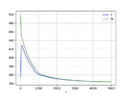
This doesn't look anything like what I expected. I was expecting to see something like the previous graph. Wasn't the initial temperature of the bed supposed to be < 80 K, and the gas temperature supposed to be about 300 K? What did you use for T1 and T2, for the inlet gas temperature, and for the bed-filled-with-liquid temperature? Also, on the graph, please show times from 0 to 1000 s only.casualguitar said:Hi Chet, phase change model code below with a graph of the fluid and solid temperatures over time. I could tweak the inputs until the graph looks nicer but in the interest of saving time I wont. Basically the code is exactly the same as the last model, except now we just take m and cp as variable rather than constant (as shown in the mass and cp functions).
View attachment 292166
View attachment 292167
View attachment 292169
So looking at the graph, initially the fluid temperature and the solid temperature jump towards one another, and then gradually both reduce to the gas inlet temperature. This happens slowly though, meaning that the mass flow in is small relative to the volume holdup. We also have the linear increase/decrease in temperature between T1 and T2 (shown by the straight line sections on the blue curve)
How does this look to you? What are your thoughts on adding in temperature variation along the direction of flow? Is this a reasonable development?
Ah my apologies, the ##80K/300K## temperatures refer to the liquefaction of air model. I just chose water/steam for the model above to test this phase change model. I've switched it now so the initial temperature of the bed and fluid in the bed are both ##80K##, and the gas entering is ##300K##. I used ##T1 = 100K## and ##T2 = 110K## to approximate a boiling range. Range adjusted to ##1000s## also. I've also switched the input values (cp, vL, etc to reflect average air properties).Chestermiller said:This doesn't look anything like what I expected. I was expecting to see something like the previous graph. Wasn't the initial temperature of the bed supposed to be < 80 K, and the gas temperature supposed to be about 300 K? What did you use for T1 and T2, for the inlet gas temperature, and for the bed-filled-with-liquid temperature? Also, on the graph, please show times from 0 to 1000 s only.
I assume you've run a range of test cases to put the model through its paces and get a feel for the quantitative effects of some of the parameters such as the heat transfer coefficient.casualguitar said:Ah my apologies, the ##80K/300K## temperatures refer to the liquefaction of air model. I just chose water/steam for the model above to test this phase change model. I've switched it now so the initial temperature of the bed and fluid in the bed are both ##80K##, and the gas entering is ##300K##. I used ##T1 = 100K## and ##T2 = 110K## to approximate a boiling range. Range adjusted to ##1000s## also. I've also switched the input values (cp, vL, etc to reflect average air properties).
View attachment 292183
My apologies for the confusion there. What are your thoughts on adding in temperature variation along the direction of flow? Is this a reasonable development?
Chestermiller said:I assume you've run a range of test cases to put the model through its paces and get a feel for the quantitative effects of some of the parameters such as the heat transfer coefficient.
Yes I've played with the input parameters to get an idea of how much of an effect it has on the output. I have got a more intuitive idea now as for how the system reacts to changes in input. Yes I would not have been able to do this with a full scale model, so really I suppose it can be faster to build simple models up gradually rather than go straight for the full version. I will incorporate this approach for future models!Chestermiller said:I'm hoping that you have developed an appreciation for the value of solving simple crude models of a system first before going to the more complicated versions. In this case, you have been able to develop a strategy for including the thermodynamics of the phase change in the calculations. Imagine having tried to do this with the full version of the model. You also have some results under your belt, so you already have a feel for the time scale of the behavior; the time for the system to be fully purged is going to be on the order of about 15 minutes. In my judgment, this has been of tremendous value. Please try to incorporate this kind of approach, in building from simple models to more complicated ones, as part of your routine strategy for the future.
Great. I'm ready for this discussion now alsoChestermiller said:We are going to need to have some discussions on expanding this to include the axial variation.
Thank you for this again, it is hugely appreciated. I won't ask too many questions yet but I thought we were avoiding manually implementing these FD schemes and instead using existing libraries to solve PDEs? I assume I'm misunderstanding what you mean by thisChestermiller said:I've been working on a finite difference scheme that I would be comfortable with for axial discretization; I'm close to finishing, and will document it for your consideration when I'm done.
Not really. Axial dispersion refers to generally undesirable heat transfer both along the direction of flow and against the direction of flow I believe? For example over time the temperature gradient in a packed bed would reduce due to the temperature differences between the high and low temperature zones. I don't know why this would be different to conduction though. I assumed it would be a combination of conduction and convection.Chestermiller said:We also need to address dealing with numerical issues associated with advection/diffusion situations like this. Are you familiar with the concept of axial dispersion (over and above conduction ) in porous media and packed beds? Are you familiar with the "method of lines" for solving partial differential equations involving time and spatial position?
Understood. I did some reading on solving PDEs with the solve_ivp package I've used above and yes they generally said something similar to what you have said.Chestermiller said:To use the package codes to solve PDEs, you need to first discretize the equations spatially, but retain the time derivatives
I have seen solutions of PDEs similar to the ones I included in my original question that use methods like Crank Nicolson etc to solve for the temperature profiles at each time increment, where both the time and space domains are discretised. Why choose the method of lines approach over an approach like this?Chestermiller said:So you will be solving a set of coupled first order ordinary differential equations in time for the temperatures as the spatial grid points. This is called the method of lines.
Hi Chet, just a quick update - I have now read up on the method of lines and have followed an example solution in MATLAB. To answer my own previous question regarding the use cases for the MOL, it seems the MOL would be chosen to take advantage of the methods and software that have been developed for numerically integrating ODEsChestermiller said:To use the package codes to solve PDEs, you need to first discretize the equations spatially, but retain the time derivatives, which now become ordinary time derivatives. So you will be solving a set of coupled first order ordinary differential equations in time for the temperatures as the spatial grid points. This is called the method of lines. The package codes automatically solve these, and certain options guarantee stability of the time integration.
Understood. I will read up on this now. Any aspects of porous media axial dispersion in particular? If not I will read up on how axial dispersion in packed beds is modeled. Thank youChestermiller said:You need to read up on axial heat dispersion in packed beds (over and above axial heat conduction). We need to discuss how to handle this.
Yes. You may have to make this an adjustable parameter when you tune your model to the experimental data.casualguitar said:I've spent the last few hours reading papers that include axial dispersion. I understand now why this isn't trivial. There are lots of correlations we could use to find a thermal axial dispersion coefficient (as a function of thermal conductivity, porosity etc).
This paper is quite similar to what we're doing, and it uses an axial dispersion coefficient correlation: https://www.sciencedirect.com/science/article/abs/pii/0038092X82902067
So essentially it seems to be 'lumped in' with the conduction term, by using a pseudoproperty ##K_Z## rather than the actual thermal conductivity.
Is this what you had in mind?
This paper doesn't seem to include a 2nd fluid phase.casualguitar said:Also while reading I found this paper, which is sort of close to what we're doing: https://www.sciencedirect.com/science/article/pii/000925097480059X?via=ihub
I will take a close read of both of these tomorrow morning to prepare for this discussion
UnderstoodChestermiller said:Yes. You may have to make this an adjustable parameter when you tune your model to the experimental data.
Yes you're absolutely right I linked the wrong one. This is the correct one: https://www.sciencedirect.com/science/article/pii/001793109090255SChestermiller said:This paper doesn't seem to include a 2nd fluid phase.
I have access to only the abstract.casualguitar said:Understood
Yes you're absolutely right I linked the wrong one. This is the correct one: https://www.sciencedirect.com/science/article/pii/001793109090255S
This paper does assume axial dispersion is negligible so it won't be of use for that. It does model two phase flow though
Ok so are you saying we will not just have two energy balance equations, but also a mass balance to the fluid equation, meaning our 'system' will involve solving three ODEs?Chestermiller said:In our analysis, a complexity in writing down the finite difference expressions for the spatial direction is that the density and mass rate of flow are both functions of time and spatial position; this needs to be accounted for in the mass balance equation and in the energy balance equation. This is what I've been working on.
Not exactly. I'll get to that soon.casualguitar said:I've set up a WeTransfer (allows sending of the PDF) link if you want to look at the paper: https://we.tl/t-9ebfBtGiuR
Yes correct they are. The library I am using can do temperature and pressure dependent parameters, this is an overview of the documentation if you want to take a look at the functionality: https://thermo.readthedocs.ioOk so are you saying we will not just have two energy balance equations, but also a mass balance to the fluid equation, meaning our 'system' will involve solving three ODEs?
Will do. Just some questions to clarify:Chestermiller said:Try modifying the stirred tank version of the numerical model by solving the fluid heat balance equation mdhdt=m˙in(hin−h)−UA(T(h)−TS) (from post #12) in terms of the enthalpy h rather than the temperate T. (The heat balance for the solid can be left in terms of T and TS).
Two phase.casualguitar said:Will do. Just some questions to clarify:
1) Am I to solve this for a single phase only, or for two phase flow?
You use the property equations for M and h that we have written for the 2 phase model. It's easiest to express T and M as functions of h over the three intervals.casualguitar said:2) The equation you supplied: ##m\frac{dh}{dt}=\dot{m}_{in}(h_{in}-h)-UA(T(h)-T_S)## seems to be in a useful form already. So if we are working on a single phase model then I actually only need an equation of state here I think, H(T) and T(H), and then we can solve using the ODE solver as usual
Is the above correct? i.e. your equation is in a useful form and I just need an EOS (thermodynamic property library) to solve?
Are we assuming ##C_{PL}## and ##C_{PG}## are constant?Chestermiller said:You use the property equations for M and H that we have written for the 2 phase model.
OK. Let's do the interval thing with this approach.casualguitar said:Are we assuming ##C_{PL}## and ##C_{PG}## are constant?
So the differences in terms of calculations here would be:
1) We are first calculating the inlet enthalpy using the previously developed property equations
2) The mass holdup will now be a function of enthalpy instead of temperature, meaning that we should solve for ##T_{sat}## in each of the three enthalpy property equations
3) At each time step we solve for the fluid ##H##, and then convert to ##H## to ##T## for input into the solid equation
4) Also we would need the enthalpy at ##T1## and ##T2## rather than the temperature bounds
I will start on this solution this evening however I'm not sure why this enthalpy model would output different results to the temperature model. Why would it?
I'll do the necessary equation adjusting and comment with a clear algorithm before I start coding