A Journey to The Manifold SU(2): Differentiation, Spheres, and Fiber Bundles

Part 2

 

Differentiation, Spheres, and Fiber Bundles

Image source: [24]

The special unitary groups play a significant role in the standard model in physics. Why? An elaborate answer would likely involve a lot of technical terms as Lie groups, Riemannian manifolds or Hilbert spaces, wave functions, generators, Casimir elements, or irreps. This already reveals that entire books could be written about them, and to be honest, they have been written about them. The many aspects are unfortunately found in quite a lot of different books, lectures, or articles. There is furthermore a gap between the language physicists use and the language mathematicians use. The former is often an abbreviation for entire contexts and the latter often hidden when used in physics. I will try to shed some light on the mathematical side of the coin, of course without claiming completeness. It is all about symmetries and derivatives at its heart. Emmy Noether’s famous theorem $[1]$ is pretty fundamental – one could easily develop entire physical and mathematical theories just as applications of Noether’s theorem. The environment to prove it takes unfortunately a while itself to be developed.

The following text is meant to make its readers curious about a group that plays a big role in physics and shed some light on its many facets. I also hope it can be used as a quick reference guide to look up certain terms, definitions, and relations, or at least as an invitation to read more, e.g. in the sources listed at the end.

1. A Real One-Parameter Local Lie Group

We start with an example of a local Lie group to demonstrate the difference to global Lie groups like $SU(2,\mathbb{C})$. An $n-$parameter local, real Lie group consists of connected open subsets $U_0 \subseteq U \subseteq \mathbb{R}^n$, a smooth group multiplication $U \times U \longrightarrow \mathbb{R}^n$ and a smooth inversion $\{0\} \in U_0 \longrightarrow U$ with $0$ as identity element and the usual group axioms. The locality is given by the fact that the group operations only need to apply in a local area around the identity element. The same holds for the group axioms: they only have to hold in small neighborhoods where they are defined. This makes it different from a global Lie group, where those operations are defined globally. On the sets $U = \{x \in \mathbb{R}\, : \,|x|< 1\}$ and $U_0 = \{x \in \mathbb{R}\, : \,|x|< \frac{1}{2}\}$ for inversion we get a locally defined Lie group by the multiplication rule $$ x \cdot y = \frac{2xy-x-y}{xy-1} $$
with the neutral element $0$ and inverse $x^{-1}=\frac{x}{2x-1}\,$. It is a one-dimensional real Lie group on $U$ which isn’t a global one. Whereas any coordinate chart of the identity element of a global Lie group defines a local Lie group, the reverse is less obvious. However, every local Lie group is locally isomorphic to a neighborhood of the neutral element of some global Lie group $[1]$.

Let’s consider the operation of left multiplication on $U$: $L_g(x) = \frac{2gx-g-x}{gx-1}$ and differentiate it
$$
\left.\frac{d}{d\,x}\right|_{x=x_0}\,L_g(x) = \frac{(g-1)^2}{(gx_0-1)^2}
$$
which can be written by the Weierstraß formulation as
\begin{equation*}
\begin{aligned}
\mathbf{f(x_{0}+v)}&=\mathbf{f(x_{0})+J(x_0;v)+r(x_0;v)} \\
L_g(x_0+v)&=L_g(x_0)+\frac{(g-1)^2}{(gx_0-1)^2}\cdot v + r(v)
\end{aligned}
\end{equation*}
where the error or remainder function $r$ has the property, that it converges faster to zero than linear, because with $$\alpha_{x_0} = \frac{(g-1)^2}{(gx_0-1)^2} \textrm{ and } \beta_{x_0}=\frac{g}{gx_0-1}$$ we have
$$
r(x_0;v)=\alpha_{x_0} \cdot (-\beta_{x_0} v^2+\beta_{x_0}^2v^3-\beta_{x_0}^3v^4+-\ldots\;) = O(v^2)
$$
So for the derivative $\alpha_{x_0}$, resp. the Jacobi matrix  $J_{x_0}$, we have beside the various notations (Newton, Leibniz, Euler, Lagrange, Jacobi, etc.) as
$$
D_{x_0}L_g(v)= (DL_g)_{x_0}(v) = \left.\frac{d}{d\,x}\right|_{x=x_0}\,L_g(x).v = J_{x_0}(L_g)(v)=J(L_g)(x_0;v)
$$
also various interpretations such as

1. first derivative $L’_g : x \longmapsto \alpha(x)$
2. differential $dL_g = \alpha_x \cdot d x$
3. linear approximation of $L_g$ by $L_g(x_0+\varepsilon)=L_g(x_0)+J_{x_0}(L_g)\cdot \varepsilon +O(\varepsilon^2)$
4. linear mapping (Jacobi matrix) $J_{x}(L_g) : v \longmapsto \alpha_{x} \cdot v$
5. vector (tangent) bundle $(p,\alpha_{p}\;d x) \in (U\times \mathbb{R},\mathbb{R},\pi)$
6. $1-$form (Pfaffian form) $\omega_{p} : v \longmapsto \langle \alpha_{p} , v \rangle$
7. cotangent bundle $(p,\omega_p) \in (U,T^*U,\pi^*)$
8. section of $(U\times \mathbb{R},\mathbb{R},\pi)\, : \,\sigma \in \Gamma(U,TU)=\Gamma(U) : p \longmapsto \alpha_{p}$
9. If $f,g : U \mapsto \mathbb{R}$ are smooth functions, then \begin{equation*}
   \begin{aligned}D_xL_y (f\cdot g) &= \alpha_x (f\cdot g)’ \\&= \alpha_x (f’\cdot g + f \cdot g’) \\&= D_xL_y(f)\cdot g + f \cdot D_xL_y(g) \end{aligned} \end{equation*} and $D_xL_y$ is a derivation on $C^\infty(\mathbb{R})$.
10. $L^*_x(\alpha_y)=\alpha_{xy}$ is the pullback section of $\sigma: p \longmapsto \alpha_p$ by $L_x$.

Since it is a one-dimensional example, the Lie structures on $U$ and its tangent space $\mathbb{R}$ are Abelian. Note that all these are dependent on the point $p=x_0$ at which the differentiation is evaluated. However, this simple example illustrates the various views possible on the one result of differentiation. They are of course not different by nature, rather different by context: analytical, geometrical, algebraical, topological, and with respect to what we consider to be variable: point of evaluation, vector being applied to, function it’s applied to, pair of both or kind of function. It is simply $J_x(L_g)$ after all as that is the reason why we differentiated $L_g$ in the first place.

2. Spheres

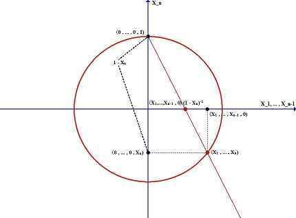
A $n-1$ sphere $\mathbb{S}^{n-1} = \{(x_1, \ldots , x_n) \in \mathbb{R}^n\, : \, x_1^2+ \ldots + x_n^2\}$ is a $n-1$ dimensional Riemannian manifold with the usual scalar product and an atlas $(U_i,\varphi_i)$

$$ U_1=\{\vec{x} \in \mathbb{S}^{n-1}\,  : \,x_n<1\} \text{ and } \varphi_1(\vec{x})=\frac{1}{1-x_n}(x_1,\ldots ,x_{n-1})$$

$$U_2=\{\vec{x} \in \mathbb{S}^{n-1}\, : \,x_n>-1\} \text{ and } \varphi_2(\vec{x})=\frac{1}{1+x_n}(x_1,\ldots ,x_{n-1})$$

where $\varphi_1$ is the stereographic projection from the north pole of the sphere onto the equatorial plane, and $\varphi_2$ the one from the south pole.

 

 

• $\mathbb{S}^0 \simeq O(1,\mathbb{R})=\{\pm 1\}$
• $\mathbb{S}^1 \simeq SO(2,\mathbb{R}) \simeq U(1,\mathbb{C}) \simeq \mathbb{P}(1,\mathbb{R}) =\text{  unit circle}$
• $\mathbb{S}^2\simeq SO(3,\mathbb{R})/SO(2,\mathbb{R}) \simeq \mathbb{P}(1,\mathbb{C}) =\text{ unit 2-sphere = Riemann sphere}$
• $\mathbb{S}^3\simeq SO(4,\mathbb{R})/SO(3,\mathbb{R}) \simeq U(1,\mathbb{H}) \simeq SU(2,\mathbb{C}) \simeq Sp(1)\simeq Spin(3) =$
  $=\text{ Principal }U(1,\mathbb{C})-\text{bundle over the 2-sphere } \mathbb{S}^2 = \text{ Hopf fibration}$
• $\mathbb{S}^4\simeq SO(5,\mathbb{R})/SO(4,\mathbb{R}) \simeq \mathbb{P}(1,\mathbb{H})$
• $\mathbb{S}^5\simeq SO(6,\mathbb{R})/SO(5,\mathbb{R}) \simeq SU(3,\mathbb{C})/SU(2,\mathbb{C}) =$
  $=\text{  Principal } U(1,\mathbb{C})\text{-bundle over }\mathbb{P}(2,\mathbb{C})$
• $\mathbb{S}^6 \simeq SO(7,\mathbb{R})/SO(6,\mathbb{R}) \simeq G_2/SU(3,\mathbb{C})$
• $\mathbb{S}^7 \simeq SO(8,\mathbb{R})/SO(7,\mathbb{R}) \simeq SU(4,\mathbb{C})/SU(3,\mathbb{C}) \simeq Sp(2)/Sp(1) \simeq Spin(7)/G_2 \simeq$ $\simeq Spin(6)/SU(3,\mathbb{C})=\text{  Principal }Sp(1)\text{-bundle over }\mathbb{S}^4$
• $\mathbb{S}^8\simeq SO(9,\mathbb{R})/SO(8,\mathbb{R}) \simeq \mathbb{P}(1,\mathbb{O})$

$\text{ Groups and Dimensions:}$

\begin{equation*}\begin{array}{cccccc} SO(n,\mathbb{R})&SU(n,\mathbb{C})&U(n,\mathbb{C})&Sp(n)&Spin(n)&G_2\\[6pt] \frac{1}{2}(n^2-n)&n^2-1&n^2&2n^2+n&\frac{1}{2}(n^2-n)&14\end{array}\end{equation*}

As we see, spheres are closely related to various symmetry groups, resp. gauge groups, resp. classical groups, resp. simple Lie groups, resp. Spin groups, resp. transformation groups which occur in physics. It’s here where all the orthogonal, unitary, Hermitian, skew-Hermitian, symplectic transformations and projective lines naturally meet.

3. The 3-Sphere or Glome or $SU(2,\mathbb{C})$

What all spheres have in common is the following short exact sequence with special orthogonal groups
\begin{equation*}
\begin{aligned}
SO(n)&=\{\,\mathbb{R}^n \stackrel{A}{\longrightarrow} \mathbb{R}^n \,: \, \langle Ax, Ay \rangle = \langle x, y \rangle \textrm{ and } \det A=1 \}\\
&=\{A\in \mathbb{M}(n,\mathbb{R}) \, : \, A \cdot A^\tau = I_n \textrm{ and } \det A=1\}
\end{aligned}
\end{equation*}
\begin{equation}\label{I}
\{1\} \rightarrow SO(n) \stackrel{\iota}{\rightarrowtail} SO(n+1) \stackrel{\pi}{\twoheadrightarrow} \mathbb{S}^n \rightarrow \{1\}
\end{equation}
where
$$\iota : A \longmapsto \begin{bmatrix} A & 0 \\ 0 & 1
\end{bmatrix} \text{ and } \pi : B \longmapsto B.\mathfrak{e}_{n+1}$$
which gives rise to the smooth bijection, the diffeomorphism $[10]$
\begin{equation}\label{II}
\mathbb{S}^{n} \simeq SO(n+1)/SO(n)
\end{equation}
To see this we can formally define the subgroup
$$H = \{A\in SO(n+1)\, :  \,A.\mathfrak{e}_{n+1}=\mathfrak{e}_{n+1}\} \leq SO(n+1)
$$
which is isomorphic to the image of $\iota$ and thus to $SO(n)$. Now the following diagram of surjective mappings
\begin{equation*}
\begin{aligned}
SO(n+1) &\stackrel{\pi}{\longrightarrow} SO(n+1)/SO(n) \\
\rho \downarrow & \quad \quad \downarrow \bar{\rho} \\
\mathbb{S}^n &\;\;= \;\; \mathbb{S}^n
\end{aligned}
\end{equation*}
defined by $(\bar{\rho}\circ \pi)(A) = \bar{\rho}(A\cdot H)=\rho(A)=A.\mathfrak{e}_{n+1}$ is commutative. The definition of $H$ makes $\bar{\rho}$ well-defined, injective and therefore a bijective mapping.

As listed above there are some more equivalent views of the 3-sphere $\mathbb{S}^3$.
$$
\mathbb{S}^3 \stackrel{\simeq_\varphi}{\longrightarrow} U(1,\mathbb{H}) \stackrel{\simeq_\psi}{\longrightarrow} SU(2,\mathbb{C}) \stackrel{\operatorname{Ad}}{\longrightarrow} SO(\mathfrak{su(2,\mathbb{C}})) \stackrel{=}{\longrightarrow} SO(3,\mathbb{R})
$$
The first two isomorphisms with
$$
\varphi(x_1\mathfrak{e}_1+x_2\mathfrak{e}_2+x_3\mathfrak{e}_3+x_4\mathfrak{e}_4)=x_1\mathbf{1}+x_2\mathbf{i}+x_3\mathbf{j}+x_4\mathbf{k} $$
and
$$
\psi(x_1\mathbf{1}+x_2\mathbf{i}+x_3\mathbf{j}+x_4\mathbf{k}) = \begin{bmatrix}x_1\mathbf{1}+x_2\mathbf{i} & -x_3\mathbf{1}+x_4\mathbf{i} \\x_3\mathbf{1}+x_4\mathbf{i} & x_1\mathbf{1}-x_2\mathbf{i} \end{bmatrix}
$$
are quite easy. Also with
\begin{equation*}
\begin{aligned}
Sp(2,\mathbb{C})
&\stackrel{def}{=}\left\{
A=\begin{bmatrix}a&b\\c&d\end{bmatrix}\in \mathbb{M}(2,\mathbb{C})\, : \,A^\tau \begin{bmatrix}0&1\\-1&0\end{bmatrix}A=\begin{bmatrix}0&1\\-1&0\end{bmatrix} \;
\right\}
\\
\\
&=\left\{
A=\begin{bmatrix}a&b\\c&d\end{bmatrix}\in \mathbb{M}(2,\mathbb{C})\, : \, ad-bc = 1 \;
\right\}
\\[6pt]
&= SL(2,\mathbb{C})
\end{aligned}
\end{equation*}
we get
$$Sp(1) = Sp(2,\mathbb{C}) \cap U(2,\mathbb{C}) = SL(2,\mathbb{C}) \cap U(2,\mathbb{C})=SU(2,\mathbb{C})$$

$Sp(1)$ stands for the compact real form of the symplectic group $Sp(2,\mathbb{C})$.

 

$SU(2,\mathbb{C})=\{X\in \mathbb{M}(2,\mathbb{C}) \,: \, \bar{X}^\tau \cdot X = I\}$ acts via the adjoint representation $\operatorname{Ad}$ on its real Lie algebra of skew-Hermitian (complex) matrices:
\begin{equation*}
\begin{aligned}
0 = D_e(I)=D_e(\bar{X}^\tau \cdot X)&=D_e(\bar{X}^\tau)\cdot X + \bar{X}^\tau \cdot D_e(X) \\ &= \bar{I}^\tau \cdot X + \bar{X}^\tau \cdot I \\&= X + \bar{X}^\tau
\end{aligned}
\end{equation*}
of $\mathfrak{su}_\mathbb{R}(2,\mathbb{C})$ via conjugation $\operatorname{Ad}: g \mapsto (X \mapsto gXg^{-1})$:
$$
\operatorname{Ad}: SU(2,\mathbb{C}) \longrightarrow SO(\mathfrak{su}_\mathbb{R}(2,\mathbb{C})) = SO(3,\mathbb{R}) \subseteq GL(3,\mathbb{R}) = GL(\mathfrak{su}_\mathbb{R}(2,\mathbb{C}))
$$
For a matrix
\begin{equation}\label{S-I}
g=g(z,w)=\begin{bmatrix}
z &-\bar{w} \\ w & \bar{z}
\end{bmatrix} \in SU(2,\mathbb{C})
\end{equation}
i.e. $|z|^2+|w|^2=1$ and with the Pauli matrices
\begin{equation}\label{S-II}
\sigma_1 = \begin{bmatrix}
0 & 1 \\ 1 & 0
\end{bmatrix}\, , \,
\sigma_2 = \begin{bmatrix}
0 & -i \\ i & 0
\end{bmatrix}\, , \,
\sigma_3 = \begin{bmatrix}
1 & 0 \\ 0 & -1
\end{bmatrix}
\end{equation}
we can define a basis $\mathfrak{B} = \{\mathfrak{e}_1,\mathfrak{e}_2,\mathfrak{e}_3\}$ by $\mathfrak{e}_k= i\cdot \sigma_k$ of $\mathfrak{su}_\mathbb{R}(2,\mathbb{C})$ and write w.r.t. $\mathfrak{B}$

\begin{equation}\label{S-III}
\operatorname{Ad}(g) = \begin{bmatrix}
\mathfrak{Re}(z^2-w^2)&\mathfrak{Im}(z^2-w^2)&2\; \mathfrak{Re}(w \cdot \bar{z})\\[6pt]
-\, \mathfrak{Im}(z^2+w^2)&\mathfrak{Re}(z^2+w^2)&2\; \mathfrak{Im}(w \cdot \bar{z})\\[6pt]
-2\; \mathfrak{Re}(w \cdot z)&-2\; \mathfrak{Im}(w \cdot z)& |z|^2-|w|^2
\end{bmatrix}
\end{equation}
The adjoint representation is surjective onto $SO(3)$ (double cover with kernel $\mathbb{Z}_2$), so there is the short exact sequence of group homomorphisms
\begin{equation}\label{III}
\{1\} \rightarrow \mathbb{Z}_2 \rightarrowtail SU(2,\mathbb{C}) \twoheadrightarrow SO(3,\mathbb{R}) \rightarrow \{1\}
\end{equation}
which shows $SU(2,\mathbb{C}) \simeq Spin(3)$ as Spin groups are the double cover of special orthogonal groups. From $(1)$ and $(2)$ we also get with the diagonal embedding of $\mathbb{Z}_2$ a short exact sequence
\begin{equation}\label{IV}
1 \rightarrow \mathbb{Z}_2 \rightarrowtail SU(2,\mathbb{C}) \times SU(2,\mathbb{C}) \simeq \mathbb{S}^3 \times \mathbb{S}^3 \twoheadrightarrow SO(4,\mathbb{R}) \rightarrow 1
\end{equation}
Note that $SU(2,\mathbb{C})$ acts on $\mathbb{C}^2$ via matrix multiplication $\operatorname{M}$ as well as on $\mathbb{R}^3$ via the adjoint representation $\operatorname{Ad}$ and we can ask, whether there is a mapping $\chi : \mathbb{C}^2 \longrightarrow \mathbb{R}^3$ such that the following diagram is commutative
\begin{equation}\label{V}
\begin{aligned}
\mathbb{C}^2 &\;\quad \stackrel{\operatorname{M}_g}{\longrightarrow} &\mathbb{C}^2\\
\downarrow{\chi}&&\downarrow{\chi}\\
\mathbb{R}^3 &\;\quad \stackrel{\operatorname{Ad} g}{\longrightarrow} &\mathbb{R}^3
\end{aligned}
\end{equation}

4. Hopf Fibration

The map $\chi : \mathbb{C}^2 \longrightarrow \mathbb{R}^3$ that makes the above diagram commutative is given by $\chi(z,w) = (\, z \bar{w}+ \bar{z} w\, , \, i\cdot (z\bar{w}- \bar{z} w)\, , \,|z|^2-|w|^2 \,)$ according to the basis $\mathfrak{B}$ and is called the Hopf map. It satisfies
$$
\chi(gv) = \chi(\operatorname{M}_g(v)) = \operatorname{Ad}(g)(\chi(v))=g \cdot\chi(v)\cdot g^{-1}
$$
for all $g \in SU(2,\mathbb{C})$ and $v \in \mathbb{C}^2$. We especially get a smooth mapping
\begin{equation}\label{VI}
\begin{aligned}
\chi \, : \, &\;\;\;\;\;\;\;\;\;\;\;\;\;\;\;\;\;\;\;\;\mathbb{S}^3 &\longrightarrow &\;\;\;\;\;\;\;\;\;\;\;\;\mathbb{S}^2\\
&(\mathfrak{Re}(z),\mathfrak{Im}(z),\mathfrak{Re}(w),\mathfrak{Im}(w))&\longmapsto&\;\;\operatorname{Ad}(g(z,w)).\mathfrak{e}_3
\end{aligned}
\end{equation}
In Cartesian and polar coordinates with $z=x+iy=(r,\varphi)=re^{i\varphi}$ and $w=u+iv=(s,\theta)=se^{i\theta}\; , \; r=\cos (\alpha), \vartheta=\theta – \varphi \;$ we get
\begin{equation}\label{VII}
\begin{aligned}
&\chi(z,w) = \chi(\begin{bmatrix} x+iy & -u+iv\\
u+iv & x-iy
\end{bmatrix}) \quad \quad \quad \quad \quad \quad \quad \quad \quad (10) \\[6pt]
&= (2(ux+vy),2(vx-uy),x^2+y^2-u^2-v^2)\\
&= (2rs \cdot \cos(\theta – \varphi),2rs \cdot \sin(\theta – \varphi), r^2-s^2) \\
&= (2\cos (\alpha)\sin (\alpha)\cos (\vartheta),2\cos (\alpha)\sin (\alpha)\sin (\vartheta),\cos^2 (\alpha)- \sin^2 (\alpha))
\end{aligned}
\end{equation}
Moreover $chi$ is a bundle projection over the basis $mathbb{S}^2$ with fiber $mathbb{S}^1$ and although $mathbb{S}^3$ isn’t the same topological space as $mathbb{S}^2 times mathbb{S}^1$, they can be identified locally. For an arbitrary point $p=(p_1,p_2,p_3) \in \mathbb{S}^2$ and $0 \leq t < 2\pi$ the fibers are for $p_3\neq -1$

\begin{equation*}
\begin{aligned}
&\chi^{-1}(p) = \sqrt{\frac{1}{2(1+p_3)}} \cdot \begin{bmatrix} i(1+p_3) &p_2+ip_1 \\
-p_2+ip_1 &-i(1+p_3)
\end{bmatrix}\cdot \begin{bmatrix} e^{it} & 0\\
0 &e^{-it}
\end{bmatrix}\\
&\\
&\chi^{-1}(p) = \sqrt{\frac{1+p_3}{2}} \cdot \begin{bmatrix} 1 & -\frac{p_1}{1+p_3}+i\frac{p_2}{1+p_3}\\
\frac{p_1}{1+p_3}+i\frac{p_2}{1+p_3} & 1
\end{bmatrix}\cdot \begin{bmatrix} e^{it} & 0\\
0 & e^{-it}
\end{bmatrix} \end{aligned} \end{equation*}

and for $p_3=-1$

\begin{equation}\label{VIII}
\chi^{-1}(0,0,-1) = \begin{bmatrix} 0 & ie^{-it}\\
ie^{it} & 0 \end{bmatrix}
\end{equation}

The Hopf bundle is even a $U(1,\mathbb{C})$ principal fiber bundle because the parameterization of the fibers by matrices of $U(1,\mathbb{C})$ can as well be used for an operation of $U(1,\mathbb{C})$ on the fibers through matrix multiplication. For a visualization of the Hopf fibration see e.g. $[13], [24]$.

5. Tangent Bundle

The Hopf fiber bundle demonstrates, that not all fiber bundles of $SU(2,\mathbb{C})$ are vector or tangent bundles, as the fiber $\mathbb{S}^1$ is no vector space. However, the Hopf fibers can be viewed as the real projective line $\mathbb{P}(1,\mathbb{R})$. Since $SU(2,\mathbb{C})$ is a smooth, analytic Lie group, its points have a tangent space spanned by the tangents of paths through them. And as a Lie group, its tangent space is a Lie algebra, $\mathfrak{su}(2,\mathbb{C})$, and the tangent bundle is built by the left-invariant vector field, i.e.
\begin{equation}\label{IX}
DL_g(\left.v\right|_h) = \left. v\right|_{L_g(h)} = \left. v\right|_{gh}
\end{equation}
Thus it is sufficient to compute the tangent space at the identity matrix $I \in G$ as we can get everywhere from there via group multiplication. For this purpose we consider a curve on $G$ and evaluate its derivative at $I$, that is a smooth function $\gamma\, : \,\mathbb{R} \longrightarrow G$ with $\gamma(0)=I$.
$$
\gamma(t) = \begin{bmatrix}
x(t)+iy(t) & -u(t)+iw(t)\\
u(t)+iw(t) & x(t)-iy(t)
\end{bmatrix}
$$
Now $\gamma(0)=I$ means $x(0)=1\, , \,y(0)=u(0)=w(0)=0$ and $\det(\gamma(t))=1$ means

\begin{equation*} \begin{aligned}
0&=\left. \frac{d}{dt}\right|_{t=0}(x^2+y^2+u^2+w^2) \\[6pt] &= 2x(0)\dot{x}(0)+2y(0)\dot{y}(0)+2u(0)\dot{u}(0)+2v(0)\dot{w}(0)
\end{aligned} \end{equation*}

and thus $\dot{x}(0)=0$. Therefore
\begin{equation}\label{X}
\begin{aligned}
D_I\gamma(t)&= \left.\dot{\gamma}(t)\right|_{t=0}\begin{bmatrix}
i\cdot\dot{y}(0) & -\dot{u}(0)+i\cdot\dot{w}(0)\\
\dot{u}(0)+i\cdot\dot{w}(0) & -i\cdot\dot{y}(0)
\end{bmatrix}\\[6pt] &= \dot{w}(0)\mathfrak{e}_1-\dot{u}(0)\mathfrak{e}_2+\dot{y}(0)\mathfrak{e}_3
\end{aligned}
\end{equation}
according to the basis $\mathfrak{B}=\{\,\mathfrak{e}_1\,,\,\mathfrak{e}_2\,,\,\mathfrak{e}_3\,\}$ of $\,T_I(SU(2,\mathbb{C}))=\mathfrak{su}(2,\mathbb{C})$.

Remember that the basis vectors $\mathfrak{e}_k=i\cdot \sigma_k$ are the $i-$multiples of the Pauli matrices.

If we consider a matrix $g=(g_{ij}) \in SU(2,\mathbb{C})$ then a vector field $v$ on it is described in local coordinates as

\begin{equation*}
\begin{aligned}
g \mapsto v|_g &= \sum_{i,j} \xi^{ij}(g) \left. \frac{\partial}{\partial x^{ij}}\right|_{x=g} &= \sum_{i,j} \xi^{ij}(g) \frac{\partial}{\partial x^{ij}} \\ &\in \left.T\, SU(2,\mathbb{C})\right|_g \\&= T_gSU(2,\mathbb{C})
\end{aligned}
\end{equation*}

A flow $\Psi(\varepsilon,g)$ passing through a point $g\in SU(2,\mathbb{C})$ generated by such a vector field $v$ is a parameterized maximal integral curve through $g$. Some examples other than the one below can be found in $[1]$. We have especially for an open interval $0 \in I \subseteq \mathbb{R}$
\begin{equation}\label{XI}
\begin{aligned}
\Psi\, : \, I \times SU(2,\mathbb{C}) &\longrightarrow SU(2,\mathbb{C})\\[6pt]
\Psi(\delta,\Psi(\varepsilon,g))&=\Psi(\delta + \varepsilon, g)\\[6pt]
\Psi(0,g)&=g\\
\frac{\partial}{\partial \varepsilon}\Psi(\varepsilon,g)&=\left.v\right|_{\Psi(\varepsilon,g)}
\end{aligned}
\end{equation}
which means $v$ is tangent to the curve $\Psi(\varepsilon,g)$ and a flow is the local group action of $\mathbb{R}$ on $SU(2,\mathbb{C})$, a one-parameter group of transformations. The vector field $v$ is called the infinitesimal generator of the action and the Taylor expansion in local coordinates $\xi = (\xi^{ij})$ for $v$ is
$$
\Psi(\varepsilon,g)=g+\varepsilon \xi(g)+O(\varepsilon^2)
$$
The computation of the flow or the real one-parameter group generated by $v$ is often called the exponentiation of $v\, : \,\exp(\varepsilon v)g \equiv \Psi(\varepsilon,g)$. This corresponds to the solution of ordinary differential equations with the help of the exponential function.

Let us consider the flow $\Psi(\varepsilon,g)$ of the left-multiplication orbit $g \mapsto \gamma(\varepsilon)\cdot g$ with
$$
\gamma(\varepsilon) = \begin{bmatrix}
e^{i\varepsilon} & 0 \\ 0 & e^{-i\varepsilon}
\end{bmatrix}
$$
With the functional equation of the exponential function only the last property in $(14)$ has to be checked:
\begin{equation*}
\begin{aligned}
\left.\frac{\partial}{\partial \varepsilon}\right|_{\varepsilon = 0}\Psi(\varepsilon,g) &= \left.\frac{\partial}{\partial \varepsilon}\right|_{\varepsilon = 0}\gamma(\varepsilon)g
= \begin{bmatrix}
i&0\\0&-i
\end{bmatrix}g = \mathfrak{e}_3\,g\\[6pt] &\stackrel{(13)}{=} D_I (\gamma(\varepsilon))\,g
\stackrel{(12)}{=} \left. v\right|_{\gamma(\varepsilon)\,g}
= \left. v\right|_{\Psi(\varepsilon, g)}
\end{aligned}
\end{equation*}

At this point the Taylor series above and the last equation in mind, it might be worth looking at the various interpretations in section $1$ again.

Sources