High Temperature and Low Duality for the Ising Model on an Infinite Regular Tree

Today I felt like sharing a computation that I thought was interesting. I’m sure I’m not the first to explore the Ising-Ising duality in this context, but I haven’t found a reference, so here we go.

The Ising model, for those uninitiated, is an idealized model of a ferromagnet. One image a crystal where each site has a free electronic spin-1/2, and there is some energy cost for neighboring spins to point in opposite directions. The classical version, where all spins are measured along some axis, say z, is already interesting. For this simple model, the spin variable on lattice site $i$ is simply a bit $s_i = \pm 1$. We write the energy of a configuration on some graph as

$$H(s) = – \sum_{\langle i j\rangle} s_i s_j$$

where $\langle i j\rangle$ denotes an edge between sites $i$ and $j$. Some materials with a privileged crystal axis actually behave according to this model!

At low temperatures in a high enough dimension (more on this in a bit), this system has an ordered phase, where the thermal average of any particular spin $\langle s_i \rangle \neq 0$. This is the phase where the material has some aggregate magnetization, with an induced magnetic field pointing along the direction of the total spin axis. This is called the ferromagnetic phase. It’s also a symmetry-broken phase, since the choice of sign of $\langle s_i \rangle$ breaks the $s_i \mapsto – s_i$ “spin-flip” symmetry of the energy $H(s)$. One should believe this at least at zero temperature by noting that the two lowest energy states are the one with all spins +1 and the one with all spins -1.

As always, however, the equilibrium is trying to minimize the free energy $F = H – TS$ rather than the true energy, so at higher temperatures $T$ we also want to maximize entropy. The all spin down and all spin up also happen to be the lowest entropy states. The magnetization with maximum entropy is the one where the number of up spins exactly balances the number of down spins. Therefore, at high temperatures we expect a phase transition to a disordered phase with $\langle s_i \rangle = 0$. In this phase, the spin-flip symmetry is restored. This is called the Curie temperature and can be reached by sticking your refrigerator magnet into your stovetop flame.

 

In one dimension, the Curie temperature is zero. There is a clever argument for this. One starts by considering, for example, the all +1 spin state. Let us call the energy of this state $H_0$. If one flips a single spin, one has two frustrated bonds which cost energy 2 each, according to our Hamiltonian above. If one flipped a whole interval of adjacent spins, the cost would be the same. All that matters are the “domain walls” between spin-up and spin-down regions. If a state has $N$ domain walls, the energy is $H_0 + 2N$. However, each domain wall can be anywhere, and so this state has $N log L$ entropy, where $L$ is the system size measured in units of lattice spacing. Thus, $F = H_0 + N(2 – T log L)$. If $T log L > 2$, $N$ tries to be as large as possible and we are in the disordered phase. Thus, as the system gets larger, the Curie temperature $T = 2/log L$ goes to zero.

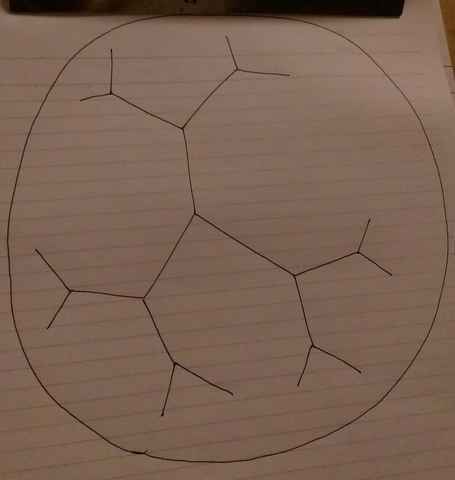
Fig. 1

It was a surprise exact calculation of the partition function of this model on a 2d square lattice that showed in 2d (and thus likely in higher dimensions) the Curie temperature is nonzero. What surprised me recently is that this system also has a finite Curie temperature on an infinite tree. The infinite tree is just some graph, so it makes sense to define the Ising model as above on its vertices. It is sometimes called a Cayley tree in analogy with the Cayley graph of a free group or sometimes in physics called the Bethe lattice. A picture is shown on the right (Fig. 1).

This picture is drawn on the Poincare model of the hyperbolic disc. It is meant to be an isometric embedding in that geometry. In particular, every point looks like every other point, and there are more and more spins as one goes closer to the hyperbolic “boundary”.

What makes the argument above not quite work for the infinite tree is that as a domain wall passes a vertex, it branches into two domain walls, doubling both the energy AND the entropy. We are in some very delicate intermediate realms with respect to the domain wall argument. Indeed, the Hausdorff dimension of this fractal tree is somewhere between 1 and 2. I’d like to ponder in what sense this is the physical dimension, but I’m not sure how…

Anyway, this phase transition is of an interesting sort. It cannot be detected by analyzing singularities of the free energy $F$. It is called an infinite-order phase transition and is similar in character to the Kosterlitz-Thouless transition in the 2d XY model. One can see it by considering applying a small magnetic field to the boundary spins at some level of finite approximation to the whole graph and then integrating out those boundary spins to get a new magnetic field and so on. Above some critical temperature, the applied magnetic field *increases* as one goes into the bulk and below that critical temperature it decreases. The latter is the ordered phase, since if one considers the reverse process, applying some small magnetic field at a site deep in the bulk, then there is a butterfly effect where that magnetic field is amplified and amplified until all the many spins near the hyperbolic boundary all point along the magnetic field. There is actually a nice problem set from some Harvard physics class that takes you through the derivation. I recommend googling for it.

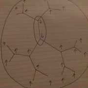
Fig. 2

I wanted to understand this phase transition more so I thought to look at the low-temperature high-temperature duality. This duality is known since 1940 by Kramers and Wannier. It is a very surprising statement already for the 2d Ising model since it relates the ordered phase at some $T<T_c$ with the disordered phase at $T_{dual} = T_c^2/T > T_c$ (note the critical model is dual to itself! it has an emergent symmetry…). To derive this duality, one expands around, say, the all spin +1 state by a sum over “droplets” of spin -1, whose energy is $H_0$ plus a term proportional to the perimeter of the droplet. This same expansion can be done on the infinite tree. An example droplet is drawn below. Each such picture represents a term in the low $T$ expansion (Fig. 2).

 

 

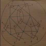
Fig. 3

Meanwhile, at high temperature, one can expand the Boltzmann weights $e^{-H/T} \simeq \prod_{\langle x y \rangle} (1 – s_x s_y/T)$ where $x, y$ denote vertices on the planar dual graph, drawn below for the infinite tree (Fig. 3).

 

 

 

 

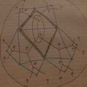
Fig. 4

Expanding the product of sums into a sum of products, one gets terms consisting of a product over $e$ many bonds weighted by $1/T^e$. It turns out these collections of bonds must form closed loops. If they have endpoints, then in the partition function when we sum over all spin configurations we will get terms that cancel in pairs. All in all, then we have a sum over loops weighted by $1/T$ to the perimeter. Thus, there is a term-by-term, order-by-order bijection between the high temperature and low-temperature expansion. With a little more work, one can identify the parameters to see how the temperature transforms. The picture below shows how to map the boundary of a low T droplet on the infinite tree to a bond loop in the high T Ising model on the dual graph (Fig. 4).

 

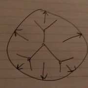
Fig. 5

This dual theory is pretty interesting because there is a natural way to map its vertices onto the hyperbolic boundary circle. This makes it almost look like a toy model of AdS/CFT, so it’s surely a good thing to try. In this 1d model, at lattice depth $k3$, lattice sites are distributed at all the $3*2^k$th roots of unity. Further, looking at a single site which without loss of generality is at 1, this site interacts with all sites of the form $\exp ( \pm 1/3*2^m)$ for $m \leq k$. In particular, the interaction strength, measured simply by the density of sites with direct interaction with our fixed site, falls off *exponentially* with distance. So this is a classical 1d system with quasilocal interaction and a finite temperature phase transition!! (Fig. 5)

 

I had never heard of such a thing, so I thought that was cool. Comments welcome!