Learn Spacetime in Mathematical Quantum Field Theory
The following is one chapter in a series on Mathematical Quantum Field Theory.
The previous chapter is 1. Geometry.
The next chapter is 3. Fields
Table of Contents
2. Spacetime
Relativistic field theory takes place in spacetime.
The concept of spacetime makes sense for every dimension ##p+1## with ##p \in \mathbb{N}##. The observable universe has macroscopic dimensions ##3+1##, but quantum field theory generally makes sense also in lower and higher dimensions. For instance, quantum field theory in dimension 0+1 is the “worldline” theory of particles, also known as quantum mechanics; while quantum field theory in dimension ##\gt p+1## may be “KK-compactified” to an “effective” field theory in dimension ##p+1## which generally looks more complicated than its higher dimensional incarnation.
However, every realistic field theory, and also most of the non-realistic field theories of interest, contain spinor fields such as the Dirac field (example 5.6 below) and the precise nature and behavior of spinors do depend sensitively on spacetime dimension. In fact, the theory of relativistic spinors is mathematically most natural in just the following four spacetime dimensions:
$$
p +1 = \phantom{AAAAA} \array{ 2+1,\; & 3+1,\; & \, & 5+1,\; &\, & \, & \, & \, 9+1 }
$$
In the literature one finds these four dimensions advertized for two superficially unrelated reasons:
- in precisely these dimensions “twistors” exist (see there);
- in precisely these dimensions “GS-superstrings” exist (see there).
However, both these explanations have a common origin in something simpler and deeper: Spacetime in these dimensions appears from the “Pauli matrices” with entries in the real normed division algebras. (In fact, it goes deeper still, but this will not concern us here.)
This we explain now, and then we use this to obtain a slick handle on spinors in these dimensions, using simple linear algebra over the four real normed division algebras. At the end (in remark 2.32) we give a dictionary that expresses these constructions in terms of the “two-component spinor notation” that is traditionally used in physics texts (remark 2.32 below).
The relation between real spin representations and division algebras is originally due to Kugo-Townsend 82, Sudbery 84, and others. We follow the streamlined discussion in Baez-Huerta 09 and Baez-Huerta 10.
A key extra structure that the spinors impose on the underlying Cartesian space of spacetime is its causal structure, which determines which points in spacetime (“events”) are in the future or the past of other points (def. 2.34 below). This causal structure will turn out to tightly control the quantum field theory on spacetime in terms of the “causal additivity of the S-matrix” (prop. 15.13 below) and the induced “causal locality” of the algebra of quantum observables (prop. 16.9 below). To prepare the discussion of these constructions, we end this chapter with some basics on the causal structure of Minkowski spacetime.
- Real division algebras
- Spacetime in dimensions 3, 4, 6 and 10
- Lorentz group and Spin group
- Spinors in dimensions 3, 4, 6 and 10
- Causal structure
Real division algebras
To amplify the following pattern and to fix our notation for algebra generators, recall these definitions:
Definition 2.1. (complex numbers)
The complex numbers ##\mathbb{C}## is the commutative algebra over the real numbers ##\mathbb{R}## which is generated from one generators ##\{e_1\}## subject to the relation
- ##(e_1)^2 = -1##.
Definition 2.2. (quaternions)
The quaternions ##\mathbb{H}## is the associative algebra over the real numbers which is generated from three generators ##\{e_1, e_2, e_3\}## subject to the relations
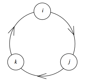
- for all ##i####(e_i)^2 = -1##
- for ##(i,j,k)## a cyclic permutation of ##(1,2,3)## then
- ##e_i e_j = e_k##
- ##e_j e_i = -e_k##
(graphics grabbed from Baez 02)
Definition 2.3. (octonions)
The octonions ##\mathbb{O}## is the nonassociative algebra over the real numbers which is generated from seven generators ##\{e_1, \cdots, e_7\}## subject to the relations
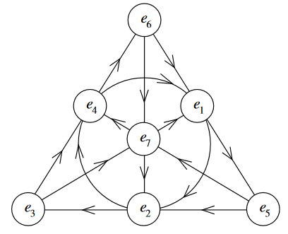
- for all ##i####(e_i)^2 = -1##
- for ##e_i \to e_j \to e_k## an edge or circle in the diagram shown (a labeled version of the Fano plane) then
- ##e_i e_j = e_k##
- ##e_j e_i = -e_k##
and all relations obtained by cyclic permutation of the indices in these equations.
(graphics grabbed from Baez 02)
One defines the following operations on these real algebras:
Definition 2.4. (conjugation, real part, imaginary part and absolute value)
For ##\mathbb{K} \in \{\mathbb{R}, \mathbb{C}, \mathbb{H}, \mathbb{O}\}##, let
$$
(-)^\ast
\;\colon\;
\mathbb{K}
\longrightarrow
\mathbb{K}
$$
be the antihomomorphism of real algebras
$$
\begin{aligned}
(r a)^\ast = r a^\ast &, \text{for}\;\; r \in \mathbb{R}, a \in \mathbb{K}
\\
(a b)^\ast = b^\ast a^\ast &,\text{for}\;\; a,b \in \mathbb{K}
\end{aligned}
$$
given on the generators of def. 2.1, def. 2.2
and def. 2.3 by
$$
(e_i)^\ast = – e_i
\,.
$$
This operation makes ##\mathbb{K}## into a star algebra. For the complex numbers ##\mathbb{C}## this is called complex conjugation, and in general we call it conjugation.
Let then
$$
Re \;\colon\; \mathbb{K} \longrightarrow \mathbb{R}
$$
be the function
$$
Re(a) \;:=\; \tfrac{1}{2}(a + a^\ast)
$$
(“real part”) and
$$
Im \;\colon\; \mathbb{K} \longrightarrow \mathbb{R}
$$
be the function
$$
Im(a) \;:= \; \tfrac{1}{2}(a – a^\ast)
$$
(“imaginary part”).
It follows that for all ##a \in \mathbb{K}## then the product of a with its conjugate is in the real center of ##\mathbb{K}##
$$
a a^\ast = a^\ast a \;\in \mathbb{R} \hookrightarrow \mathbb{K}
$$
and we write the square root of this expression as
$$
{\vert a\vert}
\;:=\;
\sqrt{a a^\ast}
$$
called the norm or absolute value function
$$
{\vert -\vert}
\;\colon\;
\mathbb{K}
\longrightarrow
\mathbb{R}
\,.
$$
This norm operation clearly satisfies the following properties (for all ##a,b \in \mathbb{K}##)
- ##\vert a \vert \geq 0##;
- ##{\vert a \vert } = 0 \;\;\;\;\; \Leftrightarrow\;\;\;\;\;\; a = 0##;
- ##{\vert a b \vert } = {\vert a \vert} {\vert b \vert}##
and hence makes ##\mathbb{K}## a normed algebra.
Since ##\mathbb{R}## is a division algebra, these relations immediately imply that each ##\mathbb{K}## is a division algebra, in that
$$
a b = 0 \;\;\;\;\;\; \Rightarrow \;\;\;\;\;\; a = 0 \;\; \text{or} \;\; b = 0
\,.
$$
Hence the conjugation operation makes ##\mathbb{K}## a real normed division algebra.
Remark 2.5. (sequence of inclusions of real normed division algebras)
Suitably embedding the sets of generators in def. 2.1, def. 2.2 and def. 2.3
into each other yields sequences of real star-algebra inclusions
$$
\mathbb{R}
\hookrightarrow
\mathbb{C}
\hookrightarrow
\mathbb{H}
\hookrightarrow
\mathbb{O}
\,.
$$
For example, for the first two inclusions, we may send each generator to the generator of the same name, and for the last inclusion I may choose
$$
\array{
1 &\mapsto& 1
\\
e_1 &\mapsto & e_3
\\
e_2 &\mapsto& e_4
\\
e_3 &\mapsto& e_6
}
$$
Proposition 2.6. (Hurwitz theorem: ##\mathbb{R}##, ##\mathbb{C}##, ##\mathbb{H}## and ##\mathbb{O}## are the normed real division algebras)
The four algebras of real numbers ##\mathbb{R}##, complex numbers ##\mathbb{C}##, quaternions ##\mathbb{H}## and octonions ##\mathbb{O}## from def. 2.1, def. 2.2 and def. 2.3 respectively, which are real normed division algebras via def. 2.4, are, up to isomorphism, the only real normed division algebras that exist.
Remark 2.7. (Cayley-Dickson construction and sedenions)
While prop. 2.6 says that the sequence from remark 2.5
$$
\mathbb{R}
\hookrightarrow
\mathbb{C}
\hookrightarrow
\mathbb{H}
\hookrightarrow
\mathbb{O}
$$
is maximal in the category of real normed non-associative division algebras, there is a pattern that does continue if one disregards the division algebra property. Namely each step in this sequence is given by a construction called forming the Cayley-Dickson double algebra. This continues to an unbounded sequence of real nonassociative star-algebras
$$
\mathbb{R}
\hookrightarrow
\mathbb{C}
\hookrightarrow
\mathbb{H}
\hookrightarrow
\mathbb{O}
\hookrightarrow
\mathbb{S}
\hookrightarrow
\cdots
$$
where the next algebra ##\mathbb{S}## is called the sedenions.
What actually matters for the following relation of the real normed division algebras to real spin representations is that they are also alternative algebras:
Definition 2.8. (alternative algebras)
Given any non-associative algebra ##A##, then the trilinear map
$$
[-,-,-] \;-\; A \otimes A \otimes A \longrightarrow A
$$
given on any elements ##a,b,c \in A## by
$$
[a,b,c] := (a b) c – a (b c)
$$
is called the associator (in analogy with the commutator ##[a,b] := a b – b a## ).
If the associator is completely antisymmetric (in that for any permutation ##\sigma## of three elements then ##[a_{\sigma_1}, a_{\sigma_2}, a_{\sigma_3}] = (-1)^{\vert \sigma\vert} [a_1, a_2, a_3]## for ##\vert \sigma \vert## the signature of the permutation) then ##A## is called an alternative algebra.
If the characteristic of the ground field is different from 2, then alternativity is readily seen to be equivalent to the conditions that for all ##a,b \in A## then
$$
(a a)b = a (a b)
\;\;\;\;\;
\text{and}
\;\;\;\;\;
(a b) b = a (b b)
\,.
$$
We record some basic properties of associators in alternative star-algebras that we need below:
Proposition 2.9. (properties of alternative star algebras)
Let ##A## be an alternative algebra (def. 2.8) which is also a star algebra. Then (using def. 2.4):
- the associator vanishes when at least one argument is real$$
[Re(a),b,c]
$$ - the associator changes sign when one of its arguments is conjugated$$
[a,b,c] = -[a^\ast,b,c]
\,;
$$ - the associator vanishes when one of its arguments is the conjugate of another$$
[a,a^\ast, b] = 0
\,;
$$ - the associator is purely imaginary$$
Re([a,b,c]) = 0
\,.
$$
Proof. That the associator vanishes as soon as one argument is real is just the linearity of an algebra product over the ground ring.
Hence in fact
$$
[a,b,c] = [Im(a), Im(b), Im(c)]
\,.
$$
This implies the second statement by linearity. And so follows the third statement by skew-symmetry:
$$
[a,a^\ast,b] = -[a,a,b] = 0
\,.
$$
The fourth statement finally follows by this computation:
$$
\begin{aligned}
\,[ a, b, c]^\ast
& =
-[c^\ast, b^\ast, a^\ast]
\\
& =
-[c,b,a]
\\
& =
-[a,b,c]
\end{aligned}
\,.
$$
Here the first equation follows by inspection and using that ##(a b)^\ast = b^\ast a^\ast##, the second follows from the first statement above, and the third is the anti-symmetry of the associator.
It is immediate to check that:
Proposition 2.10. (##\mathbb{R}##, ##\mathbb{C}##, ##\mathbb{H}## and ##\mathbb{O}## are real alternative algebras)
The real algebras of real numbers, complex numbers, def. 2.1, quaternions def. 2.2 and octonions def. 2.3 are alternative algebras (def. 2.8).
Proof. Since the real numbers, complex numbers, and quaternions are associative algebras, their associator vanishes identically. It only remains to see that the associator of the octonions is skew-symmetric. By linearity, it is sufficient to check this on generators. So let ##e_i \to e_j \to e_k## be a circle or a cyclic permutation of an edge in the Fano plane. Then by definition of the octonion multiplication we have
$$
\begin{aligned}
(e_i e_j) e_j
&=
e_k e_j
\\
&=
– e_j e_k
\\
& =
-e_i
\\
& =
e_i (e_j e_j)
\end{aligned}
$$
and similarly
$$
\begin{aligned}
(e_i e_i ) e_j
&=
– e_j
\\
&=
– e_k e_i
\\
&=
e_i e_k
\\
&=
e_i (e_i e_j)
\end{aligned}
\,.
$$
The analog of the Hurwitz theorem (prop. 2.6) is now this:
Proposition 2.11. (##\mathbb{R}##, ##\mathbb{C}##, ##\mathbb{H}## and ##\mathbb{O}## are precisely the alternative real division algebras)
The only division algebras over the real numbers which are also alternative algebras (def. 2.8) are the real numbers themselves, the complex numbers, the quaternions, and the octonions from prop. 2.10.
This is due to (Zorn 30).
For the following, the key point of alternative algebras is this equivalent characterization:
Proposition 2.12. (alternative algebra detected on subalgebras spanned by any two elements)
A nonassociative algebra is an alternative, def. 2.8, precisely if the subalgebra generated by any two elements is an associative algebra.
This is due to Emil Artin, see for instance (Schafer 95, p. 18).
Proposition 2.12 is what allows to carry over a minimum of linear algebra also to the octonions such as to yield a representation of the Clifford algebra on ##\mathbb{R}^{9,1}##. This happens in the proof of prop. 2.30 below.
So we will be looking at a fragment of linear algebra over these four normed division algebras. To that end, fix the following notation and terminology:
Definition 2.13. (hermitian matrices with values in real normed division algebras)
Let ##\mathbb{K}## be one of the four real normed division algebras from prop. 2.6, hence equivalently one of the four real alternative division algebras from prop. 2.11.
Say that an ##n \times n## matrix with coefficients in ##\mathbb{K}##
$$
A\in Mat_{n\times n}(\mathbb{K})
$$
is a hermitian matrix if the transpose matrix ##(A^t)_{i j} := A_{j i}## equals the componentwise conjugated matrix (def. 2.4):
$$
A^t = A^\ast
\,.
$$
Hence with the notation
$$
(-)^\dagger := ((-)^t)^\ast
$$
we have that ##A## is a hermitian matrix precisely if
$$
A = A^\dagger
\,.
$$
We write ##Mat_{2 \times 2}^{her}(\mathbb{K})## for the real vector space of hermitian matrices.
Definition 2.14. (trace reversal)
Let ##A \in Mat_{2 \times 2}^{her}(\mathbb{K})## be a hermitian ##2 \times 2## matrix as in def. 2.13. Its trace reversal is the result of subtracting its trace times the identity matrix:
$$
\tilde A \;:=\; A – (tr A) 1_{n\times n}
\,.
$$
Minkowski spacetime in dimensions 3,4,6 and 10
We now discover Minkowski spacetime of dimensions 3,4,6 and 10, in terms of the real normed division algebras ##\mathbb{K}## from prop. 2.6, equivalently the real alternative division algebras from prop. 2.11: this is prop./def. 2.15 and def. 2.17 below.
Proposition/Definition 2.15. (Minkowski spacetime as real vector space of hermitian matrices in real normed division algebras)
Let ##\mathbb{K}## be one of the four real normed division algebras from prop. 2.6, hence one of the four real alternative division algebras from prop. 2.11.
Then the real vector space of ##2 \times 2## hermitian matrices over ##\mathbb{K}## (def. 2.13) equipped with the inner product ##\eta## whose quadratic form ##{\vert -\vert^2_\eta}## is the negative of the determinant operation on matrices is Minkowski spacetime:
| $$ \label{MinkowskiSpacetimeFromHermitianMatricesWithDeterminant} \begin{aligned} \mathbb{R}^{dim_{\mathbb{R}}(\mathbb{K})+1,1} & := \left( \mathbb{R}^{dim_{\mathbb{R}(\mathbb{K})}+2} , {\vert -\vert^2_\eta} \right) & := \left(Mat_{2 \times 2}^{her}(\mathbb{K}), -det \right) \end{aligned} \,. $$ | (7) |
hence
- ##\mathbb{R}^{2,1}## for ##\mathbb{K} = \mathbb{R}##;
- ##\mathbb{R}^{3,1}## for ##\mathbb{K} = \mathbb{C}##;
- ##\mathbb{R}^{5,1}## for ##\mathbb{K} = \mathbb{H}##;
- ##\mathbb{R}^{9,1}## for ##\mathbb{K} = \mathbb{O}##.
Here we think of the vector space on the left as ##\mathbb{R}^{p,1}## with
$$
p := dim_{\mathbb{R}}(\mathbb{K})+1
$$
equipped with the canonical coordinates labeled ##(x^\mu)_{\mu = 0}^p##.
As a linear map the identification is given by
$$
(x^0, x^1, \cdots, x^{d-1})
\;\mapsto\;
\left(
\array{
x^0 + x^1 & y
\\
y^\ast & x^0 – x^1
}
\right)
\;\;\;
\text{with}\;
y := x^2 1 + x^3 e_1 + x^4 e_2 + \cdots + x^{2 + dim_{\mathbb{R}(\mathbb{K})}} \,e_{dim_{\mathbb{R}}(\mathbb{K})-1}
\,.
$$
This means that the quadratic form ##{\vert – \vert^2_\eta}## is given on an element ##v = (v^\mu)_{\mu = 0}^p## by
$$
{\vert v \vert}^2_{\eta}
\;=\;
– (v^0)^2 + \underset{j = 1}{\overset{p}{\sum}} (x^j)^2
\,.
$$
By the polarization identity the quadratic form ##{\vert – \vert^2_\eta}## induces a bilinear form
$$
\eta \;\colon\; \mathbb{R}^{p,1}\otimes \mathbb{R}^{p,1} \longrightarrow \mathbb{R}
$$
given by
$$
\begin{aligned}
\eta(v_1, v_2)
& =
\eta_{\mu \nu} v_1^\mu v_1^\nu
\\
& :=
– v_1^0 v_2^0 + \underset{j = 1}{\overset{p}{\sum}} v_1^j v_2^j
\end{aligned}
\,.
$$
This is called the Minkowski metric.
Finally, under the above identification the operation of trace reversal from def. 2.14
corresponds to time reversal in that
$$
\widetilde{
\left(
\array{
x^0 + x^1 & y
\\
y^\ast & x^0 – x^1
}
\right)
}
\;=\;
\left(
\array{
-x^0 + x^1 & y
\\
y^\ast & -x^0 – x^1
}
\right)
\,.
$$
Proof. We need to check that under the given identification, the Minkowski norm-square is indeed given by minus the determinant on the corresponding hermitian matrices. This follows from the nature of the conjugation operation ##(-)^\ast## from def. 2.4:
$$
\begin{aligned}
–
det
\left(
\array{
x^0 + x^1 & y
\\
y^\ast & x^0 – x^1
}
\right)
& =
-(x^0 + x^1)(x^0 – x^1)
+
y y^\ast
\\
& =
-(x^0)^2 + \underset{i = 1}{\overset{p}{\sum}} (x^i)^2
\end{aligned}
\,.
$$
Remark 2.16. (physical units of length)
As the term “metric” suggests, in application to physics, the Minkowski metric ##\eta## in prop./def. 2.15 is regarded as a measure of length: for ##v \in \Gamma_x(T \mathbb{R}^{p,1})## a tangent vector at a point ##x## in Minkowski spacetime, interpreted as a displacement from event ##x## to event ##x + v##, then
- if ##\eta(v,v) \gt 0## then$$
\sqrt{\eta(v,v)} \in \mathbb{R}
$$is interpreted as a measure for the spatial distance between ##x## and ##x + v##; - if ##\eta(v,v) \lt 0## then$$
\sqrt{-\eta(v,v)} \in \mathbb{R}
$$is interpreted as a measure for the time distance between ##x## and ##x + v##.
But for this to make physical sense, an operational prescription needs to be specified that tells the experimenter how the real number ##\sqrt{\eta(v,v)}## is to be translated into a physical distance between actual events in the observable universe.
Such an operational prescription is called a physical unit of length. For example “centimeter” ##cm## is a physical unit of length, another one is “femtometer” ##fm##.
The combined information of a real number ##\sqrt{\eta(v,v)} \in \mathbb{R}## and a physical unit of length such as meter, jointly written
$$
\sqrt{\eta(v,v)} \, cm
$$
is a prescription for finding actual distance in the observable universe. Alternatively
$$
\sqrt{\eta(v,v)} \, fm
$$
is another prescription, that translates the same real number ##\sqrt{\eta(v,v)}## into another physical distance.
But of course, they are related, since physical units form a torsor over the group ##\mathbb{R}_{\gt 0}## of non-negative real numbers, meaning that any two are related by a unique rescaling. For example
$$
fm = 10^{-13} cm
\,,
$$
with ##10^{-13} \in \mathbb{R}_{\gt 0}##.
This means that once anyone prescription of turning real numbers into spacetime distances is specified, then any other such prescription is obtained from this by rescaling these real numbers. For example
$$
\begin{aligned}
\sqrt{\eta(v,v)} \, fm
& = \left( 10^{-13} \sqrt{\eta(v,v)}\right) \,cm
\\
& =
\sqrt{ 10^{-26} \eta(v,v) } \, cm
\end{aligned}
\,.
$$
The point to notice here is that, via the last line, we may think of this as rescaling the metric from ##\eta## to ##10^{-30} \eta##.
In quantum field theory, physical units of length are typically expressed in terms of a physical unit of “action”, called “Planck’s constant” ##\hbar##, via the combination of units called the Compton wavelength
| $$ \label{ComptonWavelength} \ell_m = \frac{2\pi \hbar}{m c} \,. $$ | (8) |
parameterized, in turn, by a physical unit of mass ##m##. For the mass of the electron, the Compton wavelength is
$$
\ell_e = \frac{2\pi \hbar}{m_e c} \sim 386 \, fm
\,.
$$
Another physical unit of length parameterized by a mass ##m## is the Schwarzschild radius ##r_m := 2 m G/c^2##, where ##G## is the gravitational constant. Solving the equation
$$
\array{
& \ell_m &=& r_m
\\
\Leftrightarrow & 2\pi\hbar / m c &=& 2 m G / c^2
}
$$
for ##m## yields the Planck mass
$$
m_{P} := \tfrac{1}{\sqrt{\pi}} m_{\ell = r} = \sqrt{\frac{\hbar c}{G}}
\,.
$$
The corresponding Compton wavelength ##\ell_{m_{P}}## is given by the Planck length ##\ell_P##
$$
\ell_{P} := \tfrac{1}{2\pi} \ell_{m_P} = \sqrt{ \frac{\hbar G}{c^3} }
\,.
$$
Definition 2.17. (Minkowski spacetime as a pseudo-Riemannian Cartesian space)
Prop./def. 2.15 introduces Minkowski spacetime ##\mathbb{R}^{p,1}## for ##p+1 \in \{3,4,6,10\}## as a a vector space ##\mathbb{R}^{p,1}## equipped with a norm ##{\vert – \vert_\eta}##. The genuine spacetime corresponding to this is this vector space regaded as a Cartesian space, i.e. with smooth functions (instead of just linear maps) to it and from it (def. 1.1). This still carries one copy of ##\mathbb{R}^{p,1}## over each point ##x \in \mathbb{R}^{p,1}##, as its tangent space (example 1.12)
$$
T_x \mathbb{R}^{p,1} \simeq \mathbb{R}^{p,1}
$$
and the Cartesian space ##\mathbb{R}^{p,1}## equipped with the Lorentzian inner product from prop./def. 2.15 on each tangent space ##T_x \mathbb{R}^{p,1}## (a “pseudo-Riemannian Cartesian space”) is Minkowski spacetime as such.
We write
| $$ \label{MinkowskiVolume} dvol_\Sigma \;:=\; d x^0 \wedge d x^1 \wedge \cdots \wedge d x^p \in \Omega^{p+1}(\mathbb{R}^{p,1}) $$ | (9) |
for the canonical volume form on Minkowski spacetime.
We use the Einstein summation convention: Expressions with repeated indices indicate summation over the range of indices.
For example a differential 1-form ##\alpha \in \Omega^1(\mathbb{R}^{p,1})## on Minkowski spacetime may be expanded as
$$
\alpha = \alpha_\mu d x^\mu
\,.
$$
Moreover, we use square brackets around indices to indicate skew-symmetrization. For example a differential 2-form ##\beta \in \Omega^2(\mathbb{R}^{p,1})## on Minkowski spacetime may be expanded as
$$
\begin{aligned}
\beta
& = \beta_{\mu \nu} d x^\mu \wedge d x^\nu
\\
& = \beta_{[\mu \nu]} d x^\mu \wedge d x^\nu
\end{aligned}
$$
The identification of Minkowski spacetime (def. 2.17) in the exceptional dimensions with the generalized Pauli matrices (prop./def. 2.15) has some immediate useful implications:
Proposition 2.18. (Minkowski metric in terms of trace reversal)
In terms of the trace reversal operation ##\widetilde{(-)}## from def. 2.14, the determinant operation on hermitian matrices (def. 2.13) has the following alternative expression
$$
\begin{aligned}
-det(A) & = A \tilde A
\\
& = \tilde A A
\end{aligned}
\,.
$$
and the Minkowski inner product from prop. 2.15 has the alternative expression
$$
\begin{aligned}
\eta(A,B) & = \tfrac{1}{2}Re(tr(A \tilde B))
\\
& = \tfrac{1}{2} Re(tr(\tilde A B))
\end{aligned}
\,.
$$
(Baez-Huerta 09, prop. 5)
Proposition 2.19. (special linear group ##SL(2,\mathbb{K})## acts by linear isometries on Minkowski spacetime )
For ##\mathbb{K} \in \{\mathbb{R}, \mathbb{C}, \mathbb{H}, \mathbb{O}\}## one of the four real normed division algebras (prop. 2.6) the special linear group ##SL(2,\mathbb{K})## acts on Minkowski spacetime ##\mathbb{R}^{p,1}## in dimension ##p+1 \in \{2+1, \,3+1, \, 5+1. \, 9+1\}## (def. 2.17) by linear isometries given under the identification with the Pauli matrices in prop./def. 2.15 by conjugation:
$$
\array{
SL(2,\mathbb{K}) \times \mathbb{R}^{dim(\mathbb{K}+1,1)}
& \simeq &
SL(2, \mathbb{K}) \times Mat^{herm}_{2 \times 2}(\mathbb{K})
&\overset{}{\longrightarrow}&
Mat^{herm}_{2 \times 2}(\mathbb{K})
& \simeq &
\mathbb{R}^{dim(\mathbb{K}+1,1)}
\\
&&
(G, A) &\mapsto& G \, A \, G^\dagger
}
$$
Proof. For ##\mathbb{K} \in \{\mathbb{R}, \mathbb{C}, \mathbb{H}\}## this is immediate from matrix calculus, but we spell it out now. While the argument does not directly apply to the case ##\mathbb{K} = \mathbb{O}## of the octonions, one can check that it still goes through, too.
First we need to see that the action is well defined. This follows from the associativity of matrix multiplication and the fact that forming conjugate transpose matrices is an antihomomorphism: ##(G_1 G_2)^\dagger = G_2^\dagger G_1^\dagger##. In particular, this implies that the action indeed sends hermitian matrices to hermitian matrices:
$$
\begin{aligned}
\left(
G \, A \, G^\dagger
\right)^\dagger
& =
\underset{= G}{\underbrace{\left( G^\dagger \right)}} \, \underset{= A}{\underbrace{A^\dagger}} \, G^\dagger
\\
& =
G \, A \, G^\dagger
\end{aligned}
\,.
$$
By prop./def. 2.15 such an action is an isometry precisely if it preserves the determinant. This follows from the multiplicative property of determinants: ##det(A B) = det(A) det(B)## and their compativility with conjugate transposition: ##det(A^\dagger) = det(A^\ast)##, and finally by the assumption that ##G \in SL(2,\mathbb{K})## is an element of the special linear group, hence that its determinant is ##1 \in \mathbb{K}##:
$$
\begin{aligned}
det\left(
G \, A \, G^\dagger
\right)
& =
\underset{ = 1}{\underbrace{det(G)}} \, det(A) \, \underset{= 1^\ast = 1}{\underbrace{det(G^\dagger)}}
\\
& = det(A)
\end{aligned}
\,.
$$
In fact the special linear groups of linear isometries in prop. 2.19
are the spin groups (def. 2.26 below) in these dimensions.
exceptional spinors and real normed division algebras
| Lorentzian spacetime dimension | ##\phantom{AA}##spin group | normed division algebra | ##\,\,## brane scan entry |
| ##3 = 2+1## | ##Spin(2,1) \simeq SL(2,\mathbb{R})## | ##\phantom{A}## ##\mathbb{R}## the real numbers | super 1-brane in 3d |
| ##4 = 3+1## | ##Spin(3,1) \simeq SL(2, \mathbb{C})## | ##\phantom{A}## ##\mathbb{C}## the complex numbers | super 2-brane in 4d |
| ##6 = 5+1## | ##Spin(5,1) \simeq SL(2, \mathbb{H})## | ##\phantom{A}## ##\mathbb{H}## the quaternions | little string |
| ##10 = 9+1## | ##Spin(9,1) {\simeq} \text{“}SL(2,\mathbb{O})\text{“}## | ##\phantom{A}## ##\mathbb{O}## the octonions | heterotic/type II string |
This we explain now.
Lorentz group and spin group
Definition 2.20. (Lorentz group)
For ##d \in \mathbb{N}##, write
$$
O(d-1,1) \hookrightarrow GL(\mathbb{R}^d)
$$
for the subgroup of the general linear group on those linear maps ##A## which preserve this bilinear form on Minkowski spacetime (def 2.17), in that
$$
\eta(A(-),A(-)) = \eta(-,-)
\,.
$$
This is the Lorentz group in dimension ##d##.
The elements in the Lorentz group in the image of the special orthogonal group ##SO(d-1) \hookrightarrow O(d-1,1)## are rotations in space. The further elements in the special Lorentz group ##SO(d-1,1)##, which mathematically are “hyperbolic rotations” in a space-time plane, are called boosts in physics.
One distinguishes the following further subgroups of the Lorentz group ##O(d-1,1)##:
- the proper Lorentz group$$
SO(d-1,1) \hookrightarrow O(d-1,1)
$$is the subgroup of elements which have determinant +1 (as elements ##SO(d-1,1)\hookrightarrow GL(d)## of the general linear group); - the proper orthochronous (or restricted) Lorentz group$$
SO^+(d-1,1) \hookrightarrow SO(d-1,1)
$$is the further subgroup of elements ##A## which preserve the time orientation of vectors ##v## in that ##(v^0 \gt 0) \Rightarrow ((A v)^0 \gt 0)##.
Proposition 2.21. (connected component of Lorentz group)
As a smooth manifold, the Lorentz group ##O(d-1,1)## (def. 2.20) has four connected components. The connected component of the identity is the proper orthochronous Lorentz group ##SO^+(3,1)## (def. 2.20). The other three components are
- ##SO^+(d-1,1)\cdot P##
- ##SO^+(d-1,1)\cdot T##
- ##SO^+(d-1,1)\cdot P T##,
where, as matrices,
$$
P := diag(1,-1,-1, \cdots, -1)
$$
is the operation of point reflection at the origin in space, where
$$
T := diag(-1,1,1, \cdots, 1)
$$
is the operation of reflection in time and hence where
$$
P T = T P = diag(-1,-1, \cdots, -1)
$$
is point reflection in spacetime.
The following concept of the Clifford algebra (def. 2.22) of Minkowski spacetime encodes the structure of the inner product space ##\mathbb{R}^{d-1,1}## in terms of algebraic operation (“geometric algebra”), such that the action of the Lorentz group becomes represented by a conjugation action (example 2.24 below). In particular this means that every element of the proper orthochronous Lorentz group may be “split in half” to yield a double cover: the spin group (def. 2.26 below).
Definition 2.22. (Clifford algebra)
For ##d \in \mathbb{N}##, we write
$$
Cl(\mathbb{R}^{d-1,1})
$$
for the ##\mathbb{Z}/2##-graded associative algebra over ##\mathbb{R}## which is generated from ##d## generators ##\{\Gamma_0, \Gamma_1, \Gamma_2, \cdots, \Gamma_{d-1}\}## in odd degree (“Clifford generators”), subject to the relation
| $$ \label{RelationCliffordAlgebra} \Gamma_{a} \Gamma_b + \Gamma_b \Gamma_a = – 2\eta_{a b} $$ | (10) |
where ##\eta## is the inner product of Minkowski spacetime as in def. 2.17.
These relations say equivalently that
$$
\begin{aligned}
& \Gamma_0^2 = +1
\\
& \Gamma_i^2 = -1 \;\; \text{for}\; i \in \{1,\cdots, d-1\}
\\
& \Gamma_a \Gamma_b = – \Gamma_b \Gamma_a \;\;\; \text{for}\; a \neq b
\end{aligned}
\,.
$$
We write
$$
\Gamma_{a_1 \cdots a_p}
\;:=\;
\frac{1}{p!}
\underset{{permutations \atop \sigma}}{\sum} (-1)^{\vert \sigma\vert } \Gamma_{a_{\sigma(1)}} \cdots \Gamma_{a_{\sigma(p)}}
$$
for the antisymmetrized product of ##p## Clifford generators. In particular, if all the ##a_i## are pairwise distinct, then this is simply the plain product of generators
$$
\Gamma_{a_1 \cdots a_n}
=
\Gamma_{a_1} \cdots \Gamma_{a_n}
\;\;\;
\text{if}
\;
\underset{i,j}{\forall} (a_i \neq a_j)
\,.
$$
Finally, write
$$
\overline{(-)}
\;\colon\;
Cl(\mathbb{R}^{d-1,1})
\longrightarrow
Cl(\mathbb{R}^{d-1,1})
$$
for the algebra anti-automorphism given by
$$
\overline{\Gamma_a}
:=
\Gamma_a
$$
$$
\overline{\Gamma_a \Gamma_b}
:=
\Gamma_b \Gamma_a
\,.
$$
Remark 2.23. (vectors inside Clifford algebra)
By construction, the vector space of linear combinations of the generators in a Clifford algebra ##Cl(\mathbb{R}^{d-1,1})## (def. 2.22) is canonically identified with Minkowski spacetime ##\mathbb{R}^{d-1,1}## (def. 2.17)
$$
\widehat{(-)}
\;\colon\;
\mathbb{R}^{d-1,1}
\hookrightarrow
Cl(\mathbb{R}^{d-1,1})
$$
via
$$
x_a \mapsto \Gamma_a
\,,
$$
hence via
$$
v = v^a x_x \mapsto \hat v = v^a \Gamma_a
\,,
$$
such that the defining quadratic form on ##\mathbb{R}^{d-1,1}## is identified with the anti-commutator in the Clifford algebra
$$
\eta(v_1,v_2) = -\tfrac{1}{2}( \hat v_1 \hat v_2 + \hat v_2 \hat v_1)
\,,
$$
where on the right we are, in turn, identifying ##\mathbb{R}## with the linear span of the unit in ##Cl(\mathbb{R}^{d-1,1})##.
The key point of the Clifford algebra (def. 2.22) is that it realizes spacetime reflections, rotations and boosts via conjugation actions:
Example 2.24. (Clifford conjugation)
For ##d \in \mathbb{N}## and ##\mathbb{R}^{d-1,1}## the Minkowski spacetime of def. 2.17, let ##v \in \mathbb{R}^{d-1,1}## be any vector, regarded as an element ##\hat v \in Cl(\mathbb{R}^{d-1,1})## via remark 2.23.
Then
- the conjugation action ##\hat v \mapsto -\Gamma_a^{-1} \hat v \Gamma_a## of a single Clifford generator ##\Gamma_a## on ##\hat v## sends ##v## to its reflection at the hyperplane ##x_a = 0##;
- the conjugation action$$
\hat v \mapsto \exp(- \tfrac{\alpha}{2} \Gamma_{a b}) \hat v \exp(\tfrac{\alpha}{2} \Gamma_{a b})
$$sends ##v## to the result of rotating it in the ##(a,b)##-plane through an angle ##\alpha##.
Proof. This is immediate by inspection:
For the first statement, observe that conjugating the Clifford generator ##\Gamma_b## with ##\Gamma_a## yields ##\Gamma_b## up to a sign, depending on whether ##a = b## or not:
$$
– \Gamma_a^{-1} \Gamma_b \Gamma_a
=
\left\{
\array{
-\Gamma_b & \vert \text{if}\, a = b
\\
\Gamma_b & \vert \text{otherwise}
}
\right.
\,.
$$
Therefore for ##\hat v = v^b \Gamma_b## then ##\Gamma_a^{-1} \hat v \Gamma_a## is the result of multiplying the ##a##-component of ##v## by ##-1##.
For the second statement, observe that
$$
-\tfrac{1}{2}[\Gamma_{a b}, \Gamma_c]
=
\Gamma_a \eta_{b c} – \Gamma_b \eta_{a c}
\,.
$$
This is the canonical action of the Lorentzian special orthogonal Lie algebra ##\mathfrak{so}(d-1,1)##. Hence
$$
\exp(-\tfrac{\alpha}{2} \Gamma_{ab}) \hat v \exp(\tfrac{\alpha}{2} \Gamma_{ab})
=
\exp(\tfrac{1}{2}[\Gamma_{a b}, -])(\hat v)
$$
is the rotation action as claimed.
Remark 2.25.
Since the reflections, rotations, and boosts in example 2.24 are given by conjugation actions, there is a crucial ambiguity in the Clifford elements that induce them:
- the conjugation action by ##\Gamma_a## coincides precisely with the conjugation action by ##-\Gamma_a##;
- the conjugation action by ##\exp(\tfrac{\alpha}{4} \Gamma_{a b})## coincides precisely with the conjugation action by ##-\exp(\tfrac{\alpha}{2}\Gamma_{a b})##.
Definition 2.26. (spin group)
For ##d \in \mathbb{N}##, the spin group ##Spin(d-1,1)## is the group of even graded elements of the Clifford algebra ##Cl(\mathbb{R}^{d-1,1})## (def. 2.22) which are unitary with respect to the conjugation operation ##\overline{(-)}## from def. 2.22:
$$
Spin(d-1,1)
\;:=\;
\left\{
A \in Cl(\mathbb{R}^{d-1,1})_{even}
\;\vert\;
\overline{A} A = 1
\right\}
\,.
$$
Proposition 2.27.
The function
$$
Spin(d-1,1)
\longrightarrow
GL(\mathbb{R}^{d-1,1})
$$
from the spin group (def. 2.26) to the general linear group in ##d##-dimensions given by sending ##A \in Spin(d-1,1) \hookrightarrow Cl(\mathbb{R}^{d-1,1})## to the conjugation action
$$
\overline{A}(-) A
$$
(via the identification of Minkowski spacetime as the subspace of the Clifford algebra containing the linear combinations of the generators, according to remark 2.23)
is
- a group homomorphism onto the proper orthochronous Lorentz group (def. 2.20):$$
Spin(d-1,1) \longrightarrow SO^+(d-1,1)
$$ - exhibiting a ##\mathbb{Z}/2##-central extension.
Proof. That the function is a group homomorphism into the general linear group, hence that it acts by linear transformations on the generators follows by using that it clearly lands in automorphisms of the Clifford algebra.
That the function lands in the Lorentz group ##O(d-1,1) \hookrightarrow GL(d)## follows from remark 2.23:
$$
\begin{aligned}
\eta(\overline{A}v_1A , \overline{A} v_2 A)
&=
\tfrac{1}{2}
\left(
\left(\overline{A} \hat v_1 A\right) \left(\overline{A}\hat v_2 A\right)
+
\left(\overline{A} \hat v_2 A\right) \left(\overline{A} \hat v_1 A\right)
\right)
\\
& =
\tfrac{1}{2}
\left(
\overline{A}(\hat v_1 \hat v_2 + \hat v_2 \hat v_1) A
\right)
\\
& =
\overline{A} A \tfrac{1}{2}\left( \hat v_1 \hat v_2 + \hat v_2 \hat v_1\right)
\\
& =
\eta(v_1, v_2)
\end{aligned}
\,.
$$
That it moreover lands in the proper Lorentz group ##SO(d-1,1)## follows from observing (example 2.24) that every reflection is given by the conjugation action by a linear combination of generators, which are excluded from the group ##Spin(d-1,1)## (as that is defined to be in the even subalgebra).
To see that the homomorphism is surjective, use that all elements of ##SO(d-1,1)## are products of rotations in hyperplanes. If a hyperplane is spanned by the bivector ##(\omega^{a b})##, then such a rotation is given, via example 2.24
by the conjugation action by $$
\exp(\tfrac{\alpha}{2} \omega^{a b}\Gamma_{a b})
$$
for some ##\alpha##, hence is in the image.
That the kernel is ##\mathbb{Z}/2## is clear from the fact that the only even Clifford elements which commute with all vectors are the multiples ##a \in \mathbb{R} \hookrightarrow Cl(\mathbb{R}^{d-1,1})## of the identity. For these ##\overline{a} = a## and hence the condition ##\overline{a} a = 1## is equivalent to ##a^2 = 1##. It is clear that these two elements ##\{+1,-1\}## are in the center of ##Spin(d-1,1)##. This kernel reflects the ambiguity from remark 2.25.
Spinors in dimensions 3, 4, 6 and 10
We now discuss how real spin representations (def. 2.26) in spacetime dimensions 3,4, 6, and 10 are naturally induced from linear algebra over the four real alternative division algebras (prop. 2.6).
Definition 2.28. (Clifford algebra via normed division algebra)
Let ##\mathbb{K}## be one of the four real normed division algebras from prop. 2.6, hence one of the four real alternative division algebras from prop. 2.11.
Define a real linear map
$$
\Gamma \;\colon\; \mathbb{R}^{dim_{\mathbb{R}}(\mathbb{K})+1,1} \longrightarrow End_{\mathbb{R}}(\mathbb{K}^4)
$$
from (the real vector space underlying) Minkowski spacetime to real linear maps on ##\mathbb{K}^4##
$$
\Gamma(A)
\left(
\array{
\psi
\\
\phi
}
\right)
\;:=\;
\left(
\array{
– \tilde A \phi
\\
A \psi
}
\right)
\,.
$$
Here on the right we are using the isomorphism from prop. 2.15 for identifying a spacetime vector with a ##2 \times 2##-matrix, and we are using the trace reversal ##\widetilde(-)## from def. 2.14.
Remark 2.29. (Clifford multiplication via octonion-valued matrices)
Each operation of ##\Gamma(A)## in def. 2.28 is clearly a linear map, even for ##\mathbb{K}## being the non-associative octonions. The only point to beware of is that for ##\mathbb{K}## the octonions, then the composition of two such linear maps is not in general given by the usual matrix product.
Proposition 2.30. (real spin representations via normed division algebras)
The map ##\Gamma## in def. 2.28 gives a representation of the Clifford algebra ##Cl(\mathbb{R}^{dim_{\mathbb{R}}}(\mathbb{K}+1,1) )## (this def.), i.e of
- ##Cl(\mathbb{R}^{2,1})## for ##\mathbb{K} = \mathbb{R}##;
- ##Cl(\mathbb{R}^{3,1})## for ##\mathbb{K} = \mathbb{C}##;
- ##Cl(\mathbb{R}^{5,1})## for ##\mathbb{K} = \mathbb{H}##;
- ##Cl(\mathbb{R}^{9,1})## for ##\mathbb{K} = \mathbb{O}##.
Hence this Clifford representation induces representations of the spin group ##Spin(dim_{\mathbb{R}}(\mathbb{K})+1,1)## on the real vector spaces
$$
S_{\pm } := \mathbb{K}^2
\,.
$$
and hence on
$$
S := S_+ \oplus S_-
\,.
$$
(Baez-Huerta 09, p. 6)
Proof. We need to check that the Clifford relation
$$
\begin{aligned}
(\Gamma(A))^2
& = -\eta(A,A)1
\\
& = + det(A)
\end{aligned}
$$
is satisfied (where we used (10) and (7)). Now by definition, for any ##(\phi,\psi) \in \mathbb{K}^4## then
$$
(\Gamma(A))^2
\left(
\array{
\phi
\\
\psi
}
\right)
\;=\;
–
\left(
\array{
\tilde A(A \phi)
\\
A(\tilde A \psi)
}
\right)
\,,
$$
where on the right we have in each component ordinary matrix product expressions.
Now observe that both expressions on the right are sums of triple products that involve either one real factor or two factors that are conjugate to each other:
$$
\begin{aligned}
A (\tilde A \psi)
& =
\left(
\array{
x_0 + x_1 & y
\\
y^\ast & x_0 – x_1
}
\right)
\cdot
\left(
\array{
(-x_0 + x_1) \phi_1 + y \phi_2
\\
y^\ast \phi_1 – (x_0 + x_1)\phi_2
}
\right)
\\
& =
\left(
\array{
(-x_0^2 + x_1^2) \phi_1 + (x_0 + x_1)(y \phi_2) + y (y^\ast \phi_1) – y( (x_0 + x_1) \phi_2 )
\\
\cdots
}
\right)
\end{aligned}
\,.
$$
Since the associators of triple products that involve a real factor and those involving both an element and its conjugate vanish by prop. 2.9 (hence ultimately by Artin’s theorem, prop. 2.12). In conclusion, all associators involved vanish, so that we may rebracket to obtain
$$
(\Gamma(A))^2
\left(
\array{
\phi
\\
\psi
}
\right)
\;=\;
–
\left(
\array{
(\tilde A A) \phi
\\
(A \tilde A) \psi
}
\right)
\,.
$$
This implies the statement via the equality ##-A \tilde A = -\tilde A A = det(A)## (prop. 2.18).
Proposition 2.31. (spinor bilinear pairings)
Let ##\mathbb{K}## be one of the four real normed division algebras and ##S_\pm \simeq_{\mathbb{R}}\mathbb{K}^2## the corresponding spin representation from prop. 2.30.
Then there are bilinear maps from two spinors (according to prop. 2.30) to the real numbers
$$
\overline{(-)}(-) \;\colon\; S_+ \otimes S_-\longrightarrow \mathbb{R}
$$
as well as to ##\mathbb{R}^{dim(\mathbb{K}+1,1)}##
$$
\overline{(-)}\Gamma (-) \;\colon\; S_\pm \otimes S_{\pm}\longrightarrow \mathbb{R}^{dim(\mathbb{K}+1,1)}
$$
given, respectively, by forming the real part (def. 2.4) of the canonical ##\mathbb{K}##-inner product
$$
\overline{(-)}(-) \colon S_+\otimes S_- \longrightarrow \mathbb{R}
$$ $$
(\psi,\phi)\mapsto \overline{\psi} \phi := Re(\psi^\dagger \cdot \phi)
$$
and by forming the product of a column vector with a row vector to produce a matrix, possibly up to trace reversal (def. 2.14) under the identification ##\mathbb{R}^{dim(\mathbb{K})+1,1} \simeq Mat^{her}_{2 \times 2}(\mathbb{K})## from prop. 2.15:
$$
S_+ \otimes S_+ \longrightarrow \mathbb{R}^{dim(\mathbb{K})+1,1}
$$ $$
(\psi , \phi) \mapsto \overline{\psi}\Gamma \phi :=
\widetilde{\psi \phi^\dagger + \phi \psi^\dagger}
$$
and
$$
S_- \otimes S_- \longrightarrow \mathbb{R}^{dim(\mathbb{K}+1,1)}
$$ $$
(\psi , \phi) \mapsto {\psi \phi^\dagger + \phi \psi^\dagger}
$$
For ##A \in Mat^{her}_{2 \times 2}(\mathbb{K})## the ##A##-component of this map is
$$
\eta(\overline{\psi}\Gamma \phi, A)
=
Re (\psi^\dagger (A\phi))
\,.
$$
These pairings have the following properties
- both are ##Spin(dim(\mathbb{K})+1,1)##-equivalent;
- the pairing ##\overline{(-)}\Gamma(-)## is symmetric:
$$
\label{SpinorToVectorPairingIsSymmetric}
\overline{\psi_1} \,\Gamma\, \psi_2 = + \overline{\phi_2}\, \Gamma\, \psi_1
\phantom{AAAA}
\text{for} \phantom{AA} \psi_1, \psi_2 \in S_+ \oplus S_-
$$(11)
(Baez-Huerta 09, prop. 8, prop. 9).
Remark 2.32. (two-component spinor notation)
In the physics/QFT literature the expressions for spin representations given by prop. 2.30 are traditionally written in two-component spinor notation as follows:
- An element of ##S_+## is denoted ##(\chi_a \in \mathbb{K})_{a = 1,2}## and called a left handed spinor;
- an element of ##S_-## is denoted ##(\xi^{\dagger \dot a})_{\dot a = 1,2}## and called a right handed spinor;
- an element of ##S = S_+ \oplus S_-## is denoted
$$
\label{TwoComponentNotationForDiracSpinor}
(\psi^\alpha) = \left( (\chi_a), (\xi^{\dagger \dot a}) \right)
$$(12) and called a Dirac spinor;
and the Clifford action of prop. 2.28 corresponds to the generalized “Pauli matrices”:
- a hermitian matrix ##A \in Mat^{her}_{2\times 2}(\mathbb{K})## as in prop 2.15 regarded as a linear map ##S_- \to S_+## via def. 2.28 is denoted$$
\left(x_\mu \sigma^\mu_{a \dot a}\right)
\;:=\;
\left( \array{ x_0 + x_1 & y \\ y^\ast & x_0 – x_1 } \right) \,;
$$ - the negative of the trace-reversal (def. 2.14) of such a hermitian matrix, regarded as a linear map ##S_+ \to S_-##, is denoted$$
\left(
x_\mu \widetilde \sigma^{\mu \dot a a}
\right)
\;:=\;
–
\left( \array{ -x_0 + x_1 & y \\ y^\ast & -x_0 – x_1 } \right)
\,.
$$ - the corresponding Clifford generator ##\Gamma(A) \;\colon\; S_+ \oplus S_- \to S_+ \oplus S_-## (def. 2.28) is denoted$$
x_\mu (\gamma^\mu)_{\alpha \beta}
\;:=\;
\left(
\array{
0 & x_\mu \sigma^\mu_{a \dot b}
\\
x_\mu \widetilde \sigma^{\mu \dot a b}
}
\right)
$$ - the bilinear spinor-to-vector pairing from prop. 2.31
is written as the matrix multiplication$$
\left( \overline{\psi} \, \gamma^\mu \, \phi\right)
\;:=\;
\overline{\psi}\,\Gamma \,\phi
\,,
$$where the Dirac conjugate ##\overline{\psi}## on the left is given on ##(\psi_\alpha) = (\chi_a, \xi^{\dagger \dot c})## by$$
\label{DiracConjugate}
\begin{aligned}
\overline{\psi}
& :=
\psi^\dagger \gamma^0
\\
& =
( \xi^a, \chi^\dagger_{\dot a} )
\end{aligned}
$$(13) hence, with (12):
$$
\label{TwoComponentNotationForSpinorToVectorPairing}
\begin{aligned}
\overline{\psi_1} \,\gamma^\mu\, \psi_2
& =
\psi_1^\dagger \, \gamma^0 \gamma^\mu \, \psi_2
\\
& =
(\xi_1)^a \, \sigma^\mu_{a \dot c}\, (\xi_2)^{\dagger \dot c}
+
(\chi_1)^\dagger_{\dot a} \, \widetilde \sigma^{\mu \dot a c} \, (\chi_2)_c
\end{aligned}
$$(14)
(e.g. Dermisek I-8, Dermisek I-9)
Below we spell out the example of the Lagrangian field theory of the Dirac field in detail (example 5.6). For discussion of massive chiral spinor fields one also needs the following, here we just mention this for completeness:
Proposition 2.33. (chiral spinor mass pairing)
In dimension 2+1 and 3+1, there exists a non-trivial skew-symmetric pairing
$$
\epsilon
\;\colon\;
S \wedge S
\longrightarrow
\mathbb{R}
$$
which may be normalized such that in the two-component spinor basis of remark 2.32 we have
| $$ \label{ConjugationOfLeftRightCliffordGeneratorToRightLeft} \tilde \sigma^{\mu \dot a a} = \epsilon^{a b} \epsilon^{\dot a \dot b} \sigma^\mu_{b \dot b} \,. $$ | (15) |
Proof. Take the non-vanishing components of ##\epsilon## to be
$$
\epsilon^{1 2} = \epsilon^{\dot 1 \dot 2} = \epsilon_{21} = \epsilon_{\dot 2 \dot 1} = 1
$$
and
$$
\epsilon^{2 1} = \epsilon^{\dot 2 \dot 1} = \epsilon_{1 2} = \epsilon_{\dot 1 \dot 2} = -1
\,.
$$
With this equation (15) is checked explicitly. It is clear that ##\epsilon## thus defined is skew-symmetric as long as the component algebra is commutative, which is the case for ##\mathbb{K}## being ##\mathbb{R}## or ##\mathbb{C}##.
Causal structure
We need to consider the following concepts and constructions related to the causal structure of Minkowski spacetime ##\Sigma## (def. 2.17).
Definition 2.34. (spacelike, timelike, lightlike directions; past and future)
Given two points ##x,y \in \Sigma## in Minkowski spacetime (def. 2.17), write
$$
v := y – x \in \mathbb{R}^{p,1}
$$
for their difference, using the vector space structure underlying Minkowski spacetime.
Recall the Minkowski inner product ##\eta## on ##\mathbb{R}^{p,1}##, given by prop./def. 2.15. Then via remark 2.16 we say that the difference vector ##v## is
- spacelike if ##\eta(v,v) \gt 0##,
- timelike if ##\eta(v,v) \lt 0##,
- lightlike if ##\eta(v,v) = 0##.
If ##v## is timelike or lightlike then we say that
- ##y## is in the future of ##x## if ##y^0 – x^0 \geq 0##;
- ##y## is in the past of ##x## if ##y^0 – x^0 \leq 0##.
Definition 2.35. (causal cones)
For ##x \in \Sigma## a point in spacetime (an event), we write
$$
V^+(x), V^-(x) \subset \Sigma
$$
for the subsets of events that are in the timelike future or in the timelike past of ##x##, respectively (def. 2.34) called the open future cone and open past cone, respectively, and
$$
\overline{V}^+(x), \overline{V}^-(x) \subset \Sigma
$$
for the subsets of events that are in the timelike or lightlike future or past, respectively, called the closed future cone and closed past cone, respectively.
The union
$$
J(x) := \overline{V}^+(x) \cup \overline{V}^-(x)
$$
of the closed future cone and past, cone is called the full causal cone of the event ##x##.
More generally for ##S \subset \Sigma## a subset of events we write
$$
\overline{V}^\pm(S)
\;:=\;
\underset{x \in S}{\cup} \overline{V}^{\pm}(x)
$$
for the union of the future/past closed cones of all events in the subset.
Definition 2.36. (compactly sourced causal support)
Consider a vector bundle ##E \overset{}{\to} \Sigma## (def. 1.10) over Minkowski spacetime (def. 2.17).
Write ##\Gamma_{\Sigma}(E)## for the spaces of smooth sections (def. 1.7), and write
$$
\begin{aligned}
\Gamma_{cp}(E) & \text{compact support}
\\
\Gamma_{\Sigma,\pm cp}(E) & \text{compactly sourced future/past support}
\\
\Gamma_{\Sigma,scp}(E) & \text{spacelike compact support}
\\
\Gamma_{\Sigma,(f/p)cp}(E) & \text{future/past compact support}
\\
\Gamma_{\Sigma,tcp}(E) & \text{timelike compact support}
\end{aligned}
$$
for the subsets on those smooth sections whose support is
- (##cp##) inside a compact subset,
- (##\pm cp##) inside the closed future cone/closed past cone, respectively, of a compact subset,
- (##scp##) inside the closed causal cone of a compact subset, which equivalently means that the intersection with every (spacelike) Cauchy surface is compact (Sanders 13, theorem 2.2),
- (##fcp##) inside the past of a Cauchy surface (Sanders 13, def. 3.2),
- (##pcp##) inside the future of a Cauchy surface (Sanders 13, def. 3.2),
- (##tcp##) inside the future of one Cauchy surface and the past of another (Sanders 13, def. 3.2).
(Bär 14, section 1, Khavkine 14, def. 2.1)
Definition 2.37. (causal order)
Consider the relation on the set ##P(\Sigma)## of subsets of spacetime which says a subset ##S_1 \subset \Sigma## is not prior to a subset ##S_2 \subset \Sigma##, denoted ##S_1 \geq S_2##, if ##S_1## does not intersect the causal past of ##S_2## (def. 2.35), or equivalently that ##S_2## does not intersect the causal future of ##S_1##:
$$
\begin{aligned}
(S_1 \geq S_2)
& :=
S_1 \cap \overline{V}^-(S_2) = \emptyset
\\
& \Leftrightarrow S_2 \cap \overline{V}^+(S_1) = \emptyset
\end{aligned}
\,.
$$
If ##S_1 \geq S_2## and ##S_2 \geq S_1## we say that the two subsets are spacelike separated.
Definition 2.38. (causal complement and causal closure of subset of spacetime)
For ##S \subset X## a subset of spacetime, its causal complement ##S^\perp## is the complement of the causal cone:
$$
S^\perp \;:=\; S \setminus J_X(S)
\,.
$$
The causal complement ##S^{\perp \perp}## of the causal complement ##S^\perp## is called the causal closure. If
$$
S = S^{\perp \perp}
$$
then the subset ##S## is called a causally closed subset.
Given a spacetime ##\Sigma##, we write
$$
CausClsdSubsets(\Sigma) \;\in\; Cat
$$
for the partially ordered set of causally closed subsets, partially ordered by inclusion ##\mathcal{O}_1 \subset \mathcal{O}_2##.
Definition 2.39. (adiabatic switching)
For a causally closed subset ##\mathcal{O} \subset \Sigma## of spacetime (def. 2.38) say that an adiabatic switching function or infrared cutoff function for ##\mathcal{O}## is a smooth function ##g_{sw}## of compact support (a bump function) whose restriction to some neighbourhood ##U## of ##\mathcal{O}## is the constant function with value ##1##:
$$
Cutoffs(\mathcal{O})
\;:=\;
\left\{
g_{sw} \in C^\infty_c(\Sigma)
\;\vert\;
\underset{ {U \supset \mathcal{O}} \atop { \text{neighbourhood} } }{\exists}
\left(
g_{sw}\vert_U = 1
\right)
\right\}
\,.
$$
Often we consider the vector space space ##C^\infty(\Sigma)\langle g \rangle ## spanned by a formal variable ##g## (the coupling constant) under multiplication with smooth functions, and consider as adiabatic switching functions the corresponding images in this space,
$$
\array{
C_c^\infty(\Sigma) &\overset{\simeq}{\longrightarrow}& C_c^\infty(X)\langle g\rangle
}
$$
which are thus bump functions constant over a neighbourhood ##U## of ##\mathcal{O}## not on 1 but on the formal parameter ##g##:
$$
g_{sw}\vert_U = g
\,
$$
In this sense, we may think of the adiabatic switching as being the spacetime-dependent coupling “constant”.
The following Lemma 2.40 will be key in the derivation (proof of prop. 16.4 below) of the causal locality of the algebra of quantum observables in perturbative quantum field theory:
Lemma 2.40. (causal partition)
Let ##\mathcal{O} \subset \Sigma## be a causally closed subset (def. 2.38) and let ##f \in C^\infty_{cp}(\Sigma)## be a compactly supported smooth function which vanishes on a neighbourhood ##U \supset \mathcal{O}##, i.e. ##f\vert_U = 0##.
Then there exists a causal partition of ##f## in that there exist compactly supported smooth functions ##a,r \in C^\infty_{cp}(\Sigma)## such that
- they sum up to ##f##:$$
f = a + r
$$ - their support satisfies the following causal ordering (def. 2.37)$$
supp(a) \geq \mathcal{O} \geq supp(r)
\,.
$$
Proof idea. By assumption ##\mathcal{O}## has a Cauchy surface. This may be extended to a Cauchy surface ##\Sigma_p## of ##\Sigma##, such that this is one leaf of a foliation of ##\Sigma## by Cauchy surfaces, given by a diffeomorphism ##\Sigma \simeq (-1,1) \times \Sigma_p## with the original ##\Sigma_p## at zero. There exists then ##\epsilon \in (0,1)## such that the restriction of ##supp(f)## to the interval ##(-\epsilon, \epsilon)## is in the causal complement ##\overline{\mathcal{O}}## of the given region (def. 2.38):
$$
supp(f) \cap (-\epsilon, \epsilon) \times \Sigma_p
\;\subset\;
\overline{\mathcal{O}}
\,.
$$
Let then ##\chi \colon \Sigma \to \mathbb{R}## be any smooth function with
- ##\chi\vert_{(-1,0] \times \Sigma_p} = 1##
- ##\chi\vert_{(\epsilon,1) \times \Sigma_p} = 0##.
Then
$$
r := \chi \cdot f
\phantom{AAA}
\text{and}
\phantom{AAA}
a := (1-\chi) \cdot f
$$
are smooth functions as required.
This concludes our discussion of spin and spacetime. In the next chapter, we consider the concept of fields on spacetime.
I am a researcher in the department Algebra, Geometry and Mathematical Physics of the Institute of Mathematics at the Czech Academy of the Sciences (CAS) in Prague.
Presently I am on leave at the Max Planck Institute for Mathematics in Bonn.


Time is just a mathmatical construct to measure the motionThis is a self contradiction. Mathematical constructs cannot measure physical quantities.
What is the so what here? We can write an equation to describe anything but it does not make it true or part of our world.The "so what" here is that quantum field theory is one of the most accurate mathematical descriptions of how our world works that humanity has discovered. You are right that not all equations and mathematical structures are "true or part of our world", but the stuff that Schreiber is describing here is part of our fundamental understanding of the universe that we live in.
If you want further discussion of why quantum field theory is relevant, it would be best to start your own thread in the "General Physics" section, as this thread is for people who already understand its relevance and what to understand the theory itself more deeply. But please be mindful of the Physics Forums mission statement:
Typo in proof of example 2.23: "hatv".Ok, this is where I show my ignorance, but all this is theoretical and why I get lost with these academia discussions. Time is just a mathmatical construct to measure the motion of two or more objects relative to each other. What is the so what here? We can write an equation to describe anything but it does not make it true or part of our world.
A minor note: Urs, I imagine you being more of a geometer than an analyst, so I would say: Relativistic field theory takes place on spacetime.Okay, I changed it. But I wasn't meaning to be speaking with any mathematical perspective at this point, but instead to first say something intuitive. I suppose we all feel that we live "in" spacetime, not "on" it. No?
But anyway, I should not be using parenthetical remarks in an expositional paragraph. So I changed it to "on".
Another note is that the metric tensor on the generic spacetime ##eta## is nowhere explicitely defined as diag (-++…+) and the benefit of using it compared to the "West Coast" version diag (+–..-).I did say what the norm-square is supposed to be, but you are right that I never made explicit the induced Minkowski inner product. I have expanded now def. 2.15 to make it more explicit. Then I also added a remark 2.16 on how the metric encodes length and what this means for units of length (this will be needed later in chapter 5 to understand why mass terms come with the Compton wavelength.)
Thanks for the feedback!
Typo in proof of example 2.23: "hatv".Thanks! Fixed now.
Typo in proof of example 2.23: "hatv".
A minor note: Urs, I imagine you being more of a geometer than an analyst, so I would say: Relativistic field theory takes place on spacetime. ("on" in the exact sense of fiber bundle theory, in which the Minkowski spacetime – or a curved version of it – is the basis manifold of the fiber bundles which accommodate matter fields and gauge fields, thus, technically, one has fields "living" in their own spaces, not in spacetime.
View attachment 214630
Another note is that the metric tensor on the generic spacetime ##eta## is nowhere explicitely defined as diag (-++…+) and the benefit of using it compared to the "West Coast" version diag (+–..-).
17 more parts to enjoy coming soon! :)
Thanks for writing this excellent article.