Learn How to Solve the Cubic Equation for Dummies
Everybody learns the “quadratic formula” for solving equations of the form [itex]A x^2 + B x + C = 0[/itex], even though you don’t really need such a formula, because you can solve for [itex]x[/itex] through the technique of “completing the square”. What you need a formula for is the solution to the cubic equation: [itex]Ax^3 + Bx^2 + Cx + D = 0[/itex]. There is no obvious way that “completing the cube” makes the solution into a matter of just taking cube roots in the same way that “completing the square” solves the quadratic in terms of square roots. So how could we derive such a cubic formula? Let’s see if I can convince you that you could derive it, if you thought about it hard enough, in the right way.
We’re given [itex]A x^3 + B x^2 + C x + D = 0[/itex]. Let’s assume that [itex]A=1[/itex], so we’re interested in solving an equation of the form [itex]x^3 + B x^2 + Cx + D = 0[/itex]. (A moment’s thought will show you that if you can solve that case, you can solve the general case). So by finding a “cubic formula”, we mean finding a function [itex]f(B,C,D)[/itex] that gives the solution. However, in general, a cubic equation has three solutions. So such a function must be multi-valued, with three possible values.
In the quadratic case, the solution is [itex]x = \frac{-b \pm \sqrt{b^2 – 4ac}}{2a}[/itex]. We can rewrite this in the following form:
[itex]x = \frac{-b}{2a} + r \frac{\sqrt{b^2 – 4ac}}{2a}[/itex], where [itex]r[/itex] is either plus or minus 1, that is, one of the two solutions of [itex]r^2 = 1[/itex].
Generalizing from the quadratic case, let’s assume that the multi-valuedness comes from the three branches of the cube root function. In other words, let’s look for a function of the form:
[itex]f(B,C,D,r)[/itex]
such that you get a solution whenever the parameter [itex]r[/itex] is one of the cube-roots of 1. Let’s fix [itex]B,C,D[/itex] and consider [itex]f[/itex] as a function of [itex]r[/itex]. The simplest possible non-constant functions are polynomials. So let’s assume that [itex]f[/itex] has the form: [itex]f(r) = \alpha + \beta r + \gamma r^2[/itex] (where [itex]\alpha, \beta, \gamma[/itex] are implicitly dependent on the coefficients [itex]B,C, D[/itex] of the original cubic equaion.) Since we ultimately want [itex]r[/itex] to be a cube-root of 1, we don’t need to consider terms of the form [itex]r^3[/itex] or higher-order, because those terms are reducible to lower-order terms if [itex]r^3 = 1[/itex]
A few facts about the cube roots of 1. There are three cube roots, and they can be written in the form [itex]e^{\frac{2n\pi i}{3}}[/itex]. Concretely,
[itex]r_1 = \frac{-1}{2} + \frac{\sqrt{3}}{2} i[/itex]
[itex]r_2 = \frac{-1}{2} – \frac{\sqrt{3}}{2} i[/itex]
[itex]r_3 = 1[/itex] corresponding to [itex]n = 1, 2, 3[/itex]
We can see that [itex]r_2[/itex] is just the square of [itex]r_1[/itex], so we can just write the three solutions as:
[itex]r_1 = q[/itex]
[itex]r_2 = q^2[/itex]
[itex]r_3 = 1[/itex]
where [itex]q[/itex] is [itex]e^{\frac{2 \pi i}{3}}[/itex]. Another interesting fact about the solutions is that
[itex]r_1 + r_2 + r_3 = 0[/itex]
a fact that can be proved by substitution, or geometrically, by representing the cube roots of 1 as vectors in 2-D complex space.
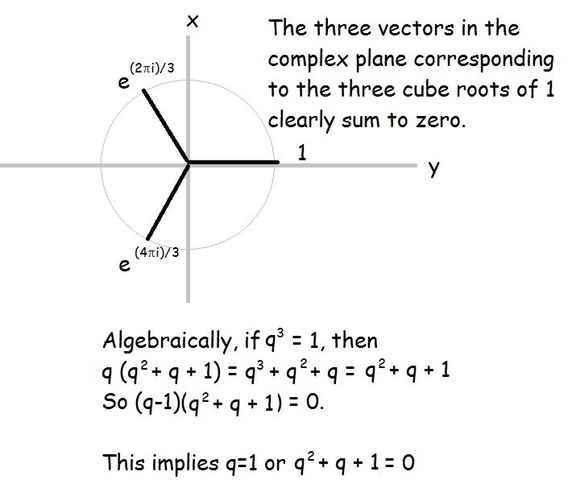
So we know that [itex]1+q+q^2 = 0[/itex] where [itex]q[/itex] is as defined.
So in terms of our function [itex]f(r)[/itex], we want the three solutions to our cubic equation to be: [itex]f(q), f(q^2), f(1)[/itex]. Using our polynomial for [itex]f[/itex], this means that we want the three solutions to be:
[itex]x_1 = \alpha + \beta q + \gamma q^2[/itex]
[itex]x_2 = \alpha + \beta q^2 + \gamma q^4 = \alpha + \beta q^2 + \gamma q[/itex]
[itex]x_3 = \alpha + \beta + \gamma[/itex]
Let’s work out a few symmetric combinations of these solutions that will be needed:
[itex]x_1 + x_2 + x_3 = 3 \alpha[/itex] (All other terms vanish, when we use the fact that [itex]1+q+q^2 = 0)[/itex]
[itex]x_1 x_2 + x_1 x_3 + x_2 x_3 = 3 (\alpha^2 – \beta \gamma)[/itex] (Again, we used [itex]1+q+q^2 = 0[/itex] to get this).
[itex]x_1 x_2 x_3 = \alpha^3 + \beta^3 + \gamma^3 – 3 \alpha \beta \gamma[/itex]
The significance of these combinations is that zeros of a polynomial can be used to factor the polynomial: If [itex]x_1, x_2, x_3[/itex] are the three solutions of [itex]x^3 + Bx^2 + Cx + D = 0[/itex], then we can write:
[itex]x^3 + Bx^2 + Cx + D = (x-x_1)(x-x_2)(x-x_3) = x^3 – (x_1 + x_2 + x_3)x^2 + (x_1 x_2 + x_1 x_3 + x_2 x_3)x – (x_1 x_2 x_3)[/itex]
Comparing coefficients tells us that
[itex](x_1 + x_2 + x_3) = -B[/itex]
[itex](x_1 x_2 + x_1 x_3 + x_2 x_3) = C[/itex]
[itex](x_1 x_2 x_3) = -D[/itex]
So using our previous results for those combinations of solutions, we find:
[itex]3 \alpha = -B[/itex]. So [itex]\alpha = \frac{-B}{3}[/itex]
[itex]3 (\alpha^2 – \beta \gamma) = C[/itex]. So [itex]\gamma = \frac{\frac{B^2}{9} – \frac{C}{3}}{\beta}[/itex]
[itex]\alpha^3 + \beta^3 + \gamma^3 – 3 \alpha \beta \gamma = -D[/itex].
In the last equation, we can substitute for [itex]\alpha[/itex] and [itex]\gamma[/itex] to get:
[itex]-\frac{B^3}{27} + D + B (\frac{B^2}{9} – \frac{C}{3}) + \beta^3 + \frac{(\frac{B^2}{9} – \frac{C}{3})^3}{\beta^3} = 0[/itex]
We can multiply by [itex]\beta^3[/itex] to get:
[itex]\beta^6 +(-\frac{B^3}{27} + D + B (\frac{B^2}{9} – \frac{C}{3})) \beta^3 + (\frac{B^2}{9} – \frac{C}{3})^3)= 0[/itex]
Oh no! After all that work to find the solution to a 3rd-degree equation, we end up with a 6th-degree equation for the coefficient [itex]\beta[/itex]. Is that progress? Well, yes it is. Because it’s only a quadratic equation in [itex]\beta^3[/itex]:
[itex](\beta^3)^2 +(-\frac{B^3}{27} + D + B (\frac{B^2}{9} – \frac{C}{3})) \beta^3 + (\frac{B^2}{9} – \frac{C}{3})^3)= 0[/itex]
So we can solve this equation for [itex]\beta^3[/itex], take the cube root of the result to get [itex]\beta[/itex] (any cube root will do), and then use the previously derived relationship between [itex]\beta[/itex] and [itex]\gamma[/itex] to find [itex]\gamma[/itex]. We already solved for [itex]\alpha[/itex]. So then we know all three coefficients in our function.
Then in terms of these values for [itex]\alpha, \beta, \gamma[/itex], we can find our three solutions to the original cubic equation:
[itex]x_1 = \alpha + \beta q + \gamma q^2[/itex]
[itex]x_2 = \alpha + \beta q^2 + \gamma q[/itex]
[itex]x_3 = \alpha + \beta + \gamma[/itex]
(where remember, q is one of the complex cube roots of 1)
I’m not going to go to the trouble of writing out the explicit solutions in terms of the coefficients of the original cubic equation. The point here is to convince you that you could compute them yourself if forced to at gunpoint.
Obviously, this general strategy for solving a polynomial equation generalizes to any degree. However, the last stroke of luck, that the 6th-degree polynomial equation for one of the coefficients can be rewritten as a quadratic equation, was unexpected. There is no reason to think that such luck will hold out for higher-degree polynomials. As a matter of fact, the French mathematician Evariste Galois, who tragically died in a duel, proved that techniques along the lines of those used here can’t be used to solve a general 5th order (or higher-order) equation.


Wow, just as nice as a musical script.
Well done stevendaryl
I actually worked out this approach years ago, on my own, but it was first discovered by the famous Lagrange, over 200 years ago:https://en.wikipedia.org/wiki/Cubic_function#Lagrange.27s_method
Great first Insight!
More!