What Are Tensors and Why Are They Used in Relativity?

If you try learning general relativity, and sometimes special relativity, on your own, you will undoubtedly run into tensors. This article will outline what tensors are and why they are so important in relativity. To keep things simple and visual, we will start in two dimensions, and in the end, generalize to more dimensions.

COORDINATE FRAMES

The essence of relativity, and thus its use of tensors, lies in coordinate frames, or frames of reference. Consider two coordinate frames, x and x’ (read as x-prime). In two dimensions, these coordinate frames have the $x_1$ and $x_{1\prime}$ axes as their respective horizontal axes, and the $x_2$ and $x_{2\prime}$ axes as their respective vertical axes. This is shown in the figure below.

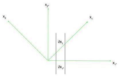
Now, we can describe an axis in one coordinate frame in terms of another coordinate frame. In the figure above, we can define the quantity $\frac{\partial x_1}{\partial x_{1\prime}}$, which is the ratio of the amount the $x_1$ axis changes in the x’ frame of reference as you change $x_{1\prime}$ an infinitesimally small amount to the infinitesimally small change you made to $x_{1\prime}$ (this is not a “normal” partial derivative in the sense that the axis of which you are taking the partial derivative is not a function. It is better to just think of it as the rate of change of an axis in one frame of reference with respect to another axis in another frame of reference). This is essentially the rate of change of $x_1$ with respect to $x_{1\prime}$. If $x_1$ were at a 45 degree angle to $x_{1\prime}$, using Pythagorean Theorem we know that this rate of change is $\sqrt{2}$. This rate of change expression, and its reciprocal, will be useful when changing frames of reference. Note that for many cases, it is essential to remember that the $\partial$ refers to an infinitesimally small change in something, as axes will not always be just straight lines with respect to another reference frame.

When working in different coordinate frames, as we do throughout physics, we need to use quantities that can be expressed in any coordinate frame– this is because any equation using those quantities is the same in any coordinate frame. Those quantities happen to be tensors. But, that definition of tensors also fits ordinary numbers (scalars) and vectors. In fact, those, too are tensors. Scalars are called rank-0 tensors, and vectors are called rank-1 tensors. For the most part, when dealing with inertial (non-accelerating) coordinates, vectors and scalars work just fine. However, when you start accelerating and curving spacetime, you need something else to keep track of that extra information. That is where higher-rank tensors come into play, namely, but not exclusively, rank-2 tensors.

VECTORS

The first step in really understanding the general idea of a tensor is by understanding vectors. 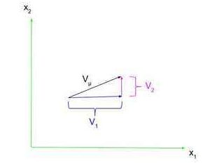A vector is defined as something with both a magnitude and direction, such as velocity or force. These vectors are often represented as a line segment with an arrowhead on one side. As shown on the right, a vector $V_{\mu}$ has components in the $x_1$ and $x_2$ directions, $V_1$ and $V_2$, respectively (note that these are just numbers, not vectors, because we already know the component vector’s direction). We can express $V_{\mu}$ in terms of its components using row vector notation, where $$V_{\mu}=\begin{pmatrix}V_1 & V_2\end{pmatrix}$$or using column vector notation, where $$V_{\mu}=\begin{pmatrix}V_1\\V_2\end{pmatrix}$$Note that we are not going to be so concerned with the position of a vector; we are just going to focus on its representation as a row or column vector.

 

TENSORS

We can now generalize vectors to tensors. Specifically, we will be using rank-2 tensors (remember, scalars are rank-0 tensors and vectors are rank-1 tensors, but when I say tensor, I am referring to rank-2 tensors). These tensors are represented by a matrix, which, in 2 dimensions, would be a 2×2 matrix. Now, we must use 2 subscripts, the first representing the row and the second representing the column. In 2 dimensions, $$T_{\mu \nu}=\begin{pmatrix}T_{11} & T_{12}\\ T_{21} & T_{22}\end{pmatrix}$$Note that each component of vectors and tensors are scalars.

You may have noticed that the rank of a tensor is shown by the number of indices on it. A scalar, S, has no indices (as there is only one component and thus no rows or columns) and is thus a rank-0 tensor; a vector, $V_{\mu}$, has 1 index and is thus a rank-1 tensor, and a rank-2 tensor, $T_{\mu\nu}$, has 2 indices as it is a rank-2 tensor. You can also see how vector/tensor components are scalars; although they have indices, they don’t have any indices that can take on different values.

THE METRIC TENSOR

There is a special tensor used often in relativity called the metric tensor, represented by $g_{\mu \nu}$. This rank-2 tensor essentially describes the coordinate system used, and can be used to determine the curvature of space. For Cartesian coordinates in 2 dimensions, or a coordinate frame with straight and perpendicular axes, $$g_{\mu \nu}=\begin{pmatrix}1 & 0\\ 0 & 1\end{pmatrix}$$which is called the identity matrix. If we switch to a different coordinate system, the metric tensor will be different. For example, for polar coordinates, $(r,\theta)$, $$g_{\mu \nu}=\begin{pmatrix}1 & 0\\ 0 & r^2\end{pmatrix}$$

DOT PRODUCTS AND THE SUMMATION CONVENTION

Take two vectors, $V^{\mu}$ and $U^{\nu}$ (where $\mu$ and $\nu$ are superscripts, not exponents. Just like subscripts, these superscripts are indices on the vectors). We can take the dot product of these two vectors, by taking the sum of the products of corresponding vector components. That is, in 2 dimensions, $$V^{\mu} \cdot U^{\nu}=V^1U^1+V^2U^2$$It is clear to see how this can be generalized to higher dimensions. However, this only works in Cartesian coordinates. To generalize this to any coordinate system, we say that $$V^{\mu} \cdot U^{\nu}=g_{\mu \nu}V^{\mu}U^{\nu}$$To evaluate this, we use the Einstein summation convention, where you sum over all indices that appear in both the top and bottom (in this case both $\mu$ and $\nu$). In two dimensions that would mean $$V^{\mu} \cdot U^{\nu}=g_{11}V^{1}U^{1}+g_{21}V^{2}U^{1}+g_{22}V^{2}U^{2}+g_{12}V^{1}U^{2}$$where we have summed up terms with every possible combination of the summed up indices (in 2 dimensions). This summation convention essentially cancels out a superscript-subscript pair. You can see that because we are only dealing with tensor and vector components, which are just scalars, the dot product of two vectors is a scalar. In Cartesian coordinates, because $g_{12}$ and $g_{21}$ are zero and $g_{11}$ and $g_{22}$ are one, we get our original definition of the dot product in Cartesian coordinates.

We can also use this convention within the same tensor. For example, there is a tensor used in general relativity called the Riemann tensor, $R^{\rho}_{\mu \rho \nu}$, a rank-4 tensor (as it has 4 indices), that can be contracted to $R_{\mu \nu}$, a rank-2 tensor, by summing over the $\rho$ which shows up as both a superscript and a subscript. That is, in 2 dimensions, $$R^{\rho}_{\mu \rho \nu}\equiv R^1_{\mu 1 \nu}+R^2_{\mu 2 \nu}=R_{\mu \nu}$$

VECTOR AND TENSOR TRANSFORMATIONS

Now that you know what a tensor is, the big question is: why are they used in relativity? This is because, by definition, tensors can be expressed in any frame of reference. Because of this, any equations using just tensors hold up in any frame of reference. Relativity is all about physics in different frames of reference, and thus it is important to use tensors, which can be expressed in any frame of reference. But, how do we transform a vector from one frame of reference to another? We will not be focusing on transforming scalars between frames of reference. Instead, we will focus on transforming vectors and rank-2 tensors. Using this, we can also discover a difference between covariant (indices as subscripts) and contravariant (indices as superscripts) tensors.

First, we can transform the vector $V_{\mu}$ into the vector $V_{\mu\prime}$. Note that these are the same vector, just one is in the “unprimed” coordinate system and one is in the “primed” coordinate system. If a dimension in the primed frame of reference changes with respect to a dimension in the unprimed frame of reference, the vector components in the two frames of reference for those dimensions should be related. Or, if the $x_{1\prime}$ dimension can be described in the x frame of reference by the $x_1$ and $x_2$ dimensions, then $V_{1\prime}$ (the vector component of the $x_{1\prime}$ axis) should be described by the relationship between the $x_{1\prime}$ dimension and the $x_1$ and $x_2$ dimensions, as well as the vector components of those dimensions ($V_1$ and $V_2$). So, our transformation equations must transform each component of $V_{\mu\prime}$ by expressing it in terms of all dimensions and vector components in the unprimed frame of reference (as any dimension in the primed frame of reference can have a relationship with all of the unprimed dimension, which we must account for). Thus, we sum over all unprimed indices, so for each component of $V_{\mu\prime}$ we have a term for each vector component in the unprimed frame of reference and their axis’s relationship to the $x_{\mu\prime}$ axis. The covariant vector transformation is thus $$V_{\mu\prime}=( \partial x_{\mu} / \partial x_{\mu\prime})V_{\mu}$$and summing over the unprimed indices in 2 dimensions, we get $$V_{\mu\prime}=( \partial x_{\mu} / \partial x_{\mu\prime})V_{\mu}=( \partial x_{1} / \partial x_{\mu\prime})V_{1}+( \partial x_{2} / \partial x_{\mu\prime})V_{2}$$To change from $V^{\mu}$ to $V^{\mu\prime}$ we use a similar equation, but we actually use the reciprocal of the derivative term used in the covariant transformation. That is, $$V^{\mu\prime}=( \partial x_{\mu\prime} / \partial x_{\mu})V^{\mu}$$and the unprimed indices are summed over as they were before. This is the contravariant vector transformation.

To transform rank-2 tensors, we do something similar, but we must adapt to having 2 indices. For a covariant tensor, to change from $T_{\mu\nu}$ to $T_{\mu\prime\nu\prime}$, $$T_{\mu\prime\nu\prime}=(\partial x_{\mu}/\partial x_{\mu\prime})(\partial x_{\nu}/\partial x_{\nu\prime})T_{\mu\nu}$$and summing over the unprimed indices in two dimensions, we get $$T_{\mu\prime\nu\prime}=(\partial x_{\mu}/\partial x_{\mu\prime})(\partial x_{\nu}/\partial x_{\nu\prime})T_{\mu\nu}=(\partial x_{1}/\partial x_{\mu\prime})(\partial x_{1}/\partial x_{\nu\prime})T_{11}+(\partial x_{1}/\partial x_{\mu\prime})(\partial x_{2}/\partial x_{\nu\prime})T_{12}+(\partial x_{2}/\partial x_{\mu\prime})(\partial x_{1}/\partial x_{\nu\prime})T_{21}+(\partial x_{2}/\partial x_{\mu\prime})(\partial x_{2}/\partial x_{\nu\prime})T_{22}$$For contravariant tensors, we once again use the reciprocal of the derivative term. To change from $T^{\mu\nu}$ to $T^{\mu\prime\nu\prime}$, we use $$T^{\mu\prime\nu\prime}=(\partial x_{\mu\prime}/\partial x_{\mu})(\partial x_{\nu\prime}/\partial x_{\nu})T^{\mu\nu}$$where the indices are summed over the same way as before.

Though the mechanics of these transformations are fairly complicated, the important part is that we can have transformation equations, and thus tensors are crucial to physics where we need to work in different coordinate frames.

GENERALIZING

We have so far been doing everything in 2 dimensions, but, as you know, the world does not work in two dimensions. It is fairly easy, though, to transform what we know in two dimensions into many dimensions.  First of all, vectors are not restricted to 2 components; in 3 dimensions they have 3 components, in 4 dimensions they have 4 components, etc. Similarly, rank-2 tensors are not always 2×2 matrices. In n dimensions, a rank-2 tensor is an nxn matrix. In each of these cases, the number of dimensions are essentially the number of different values the indices on vectors and tensors can take on (i.e. in 2 dimensions the indices can be 1 or 2, in 3 dimensions the indices can be 1, 2 or 3, etc.). Note that often for 4 dimensions, the indices can take on the values 0, 1, 2, or 3, but it is still 4 dimensional because there are 4 possible values the indices can take on, even though one of those values is 0. It is purely a matter of convention.

We must also generalize the summation convention to more dimensions. When summing over an index, you just need to remember to sum over all possible values of that index. For example, if summing over both $\mu$ and $\nu$ in 3 dimensions, you must include terms for $\mu=1$ and $\nu=1$; $\mu=2$ and $\nu=1$; $\mu=3$ and $\nu=1$; $\mu=2$ and $\nu=1$; $\mu=2$ and $\nu=2$; $\mu=2$ and $\nu=3$; $\mu=3$ and $\nu=1$; $\mu=3$ and $\nu=2$; and $\mu=3$ and $\nu=3$. Or, in the example with the Riemann tensor, in r dimensions the equation would be $$R^{\rho}_{\mu \rho \nu}\equiv R^1_{\mu 1 \nu}+R^2_{\mu 2 \nu}+R^3_{\mu 3 \nu}+…+R^r_{\mu r \nu}=R_{\mu \nu}$$

Finally, we can also generalize the transformation equations, not only to more dimensions but to different ranks of tensors. When transforming a tensor, you just need derivative terms for each index. You can also transform tensors with both covariant and contravariant indices. For example, for a tensor with one contravariant and two covariant indices, the transformation equation is $$T_{\mu\prime\nu\prime}^{\xi\prime}=(\partial x_{\mu}/\partial x_{\mu\prime})(\partial x_{\nu}/\partial x_{\nu\prime})(\partial x_{\xi\prime}/\partial x_{\xi})T_{\mu\nu}^{\xi}$$where, as you can see, the contravariant transformation derivative (with the primed coordinate on top) is used for $\xi$ and the covariant transformation derivative (with the unprimed term on top) is used for $\mu$ and $\nu$. The unprimed indices are summed over as per usual.