Series in Mathematics: From Zeno to Quantum Theory

Introduction

Series play a decisive role in many branches of mathematics. They accompanied mathematical developments from Zeno of Elea ($5$-th century BC) and Archimedes of Syracuse ($3$-th century BC), to the fundamental building blocks of calculus from the $17$-th century on, up to modern Lie theory which is crucial for our understanding of quantum theory. Series are probably the second most important objects in mathematics after functions. And the latter have often been expressed by series, especially in analysis. The term analytical function or holomorphic function represents such an identification.

A series itself is just an expression
$$
\sum_{n=1}^\infty a_n =a_1+a_2+\ldots+a_n+\ldots
$$
but this simple formula is full of possibilities. It foremost contains some more or less obvious questions:

1. Do we always have to start counting at one?
2. What does infinity mean?
3. Where are the $a_n$ from?
4. Can we meaningfully assign a value $\displaystyle{\sum_{n=1}^\infty a_n=c}$?
5. If such a value exists, will it be of the same kind?

The first question is supposedly easy to answer. No, we do not have to start with $n=1.$ We most often start at $n=0,$ sometimes at a negative integer $n=-N,$ and even $n=-\infty$ is a feasible “starting point” in some cases, creating a second infinity instead of explaining the one at the upper end that we already have.

Infinity is primarily only the notation that we do not stop with whatever we are adding here. Whether this endeavor makes sense is an entirely different question. Nevertheless, we need to define it somehow so that we can work with it. The infinity of a series is explained by the infinity of its sequence of partial sums
$$
S_m=\sum_{n=1}^m a_n \; \;(m\in \mathbb{N})
$$
and the series value $c$ is defined by its limit
$$
\sum_{n=1}^\infty a_n =\lim_{m \to \infty} S_m.
$$
The definition doesn’t say anything about the value of this limit, not even whether it exists or not. E.g.
$$
\sum_{n=1}^\infty (-1)^n=-1+1-1+1\mp \ldots {{ \nearrow \phantom{-}0}\atop{\searrow -1}}
$$
is defined as $\lim_{m \to \infty} \sum_{n=1}^m (-1)^n$ but we cannot assign a value $c$ in this case. The point of view by partial sums reduces series to ordinary sequences. Unfortunately, it disguises the important property of addition. We actually have a recursion
\begin{align*}
S_0=0\, , \,S_{m+1}=S_m+a_{m+1}.
\end{align*}
Although it is one of the simplest recursion rules that can be imagined, it contains the problem of adding infinitely often, which cannot be done in reality. At least it defines the empty sum
$$
\sum_{n\in \emptyset}a_n=\sum_{n=1}^0a_n=0
$$
which makes sense from the logical perspective since zero is the neutral element of addition: the number we use if there is no addition. But what if we actually add something, say numbers?
$$
\sum_{n=1}^\infty a_n = \begin{cases}0&\text{ if }a_n=0\quad\text{convergence} \\ \text{?}&\text{ if }a_n=1\quad\text{divergence}\end{cases}
$$
Some authors write $\displaystyle{\sum_{n=1}^\infty 1}=\infty$ but infinity is not really a value, it is no number anymore, it changed kind. Others speak of determined divergent in contrast to the case above where the potential value flips between $-1$ and $0$ which would be undetermined divergent. Anyway, the crucial questions are: Will we get closer and closer to a certain value (or plus-minus infinity) if we keep adding $a_n$? What does closer and closer mean? How do we measure distances if the series members are not numbers? What does addition mean in such a case? It leads us directly to the remaining questions and here is where the mathematics of series starts.

The series members $a_n$ can be a lot of objects. We don’t even need to actively add them, formal sums like p-adic numbers or formal power series are feasible examples where addition does not really take place. Most series, however, have members that can be added, e.g. numbers, vectors, functions, operators, or integrals to name a few. These series – other than p-adic numbers or formal power series where the assigned value of a series is basically just a name in order to deal with them – bear the question of whether they converge to a certain value that is again of the same kind as the series members. The same kind is another hidden trap. The definition of a series as a sequence of partial sums confronts us automatically with the problem that all converging sequences have. Even if the sequence members get closer and closer to each other by an increasing index, does the boundary they approach exist? The Leibniz series of rational numbers …
$$
\sum_{n=1}^{\infty }{\dfrac {(-1)^{n-1}}{2n-1}}= 1-{\dfrac{1}{3}}+{\dfrac{1}{5}}-{\dfrac{1}{7}}+{\dfrac{1}{9}}-\dotsb ={\dfrac{\pi }{4}}
$$
… converges to $\pi/4$ which is no longer a rational number. The existence of limits, i.e. the completion of topological spaces, makes the difference between rational and real numbers, pre-Hilbert and Hilbert spaces. It also means that we need a distance, a metric to measure what nearby means. Remember that the definition of a finite limit $c$ as assigned quantity to the series is
$$
\forall \;\varepsilon >0\;\exists\;N(\varepsilon)\in \mathbb{N}\;\forall \;m>N(\varepsilon )\, : \,\left|S_m-c\right|=\left|\;\sum_{n=1}^m\;a_n-\;c\; \right|<\varepsilon .
$$
We can take the absolute value in case we deal with e.g. real numbers, but vectors and functions require some thought on how we will measure the distance to the limit. All requirements together, addition, a metric, and completeness demonstrate the importance of complete topological vector spaces with a metric, Banach spaces.

Zeno of Elea, Archimedes of Syracuse,
and John von Neumann of Budapest

The easy answer about infinity isn’t as easy as it seems to be if we take a closer look. The Greek philosopher Zeno of Elea ($490–430$ BC) stated the following paradox known as Achilles and the tortoise. Achilles runs against a tortoise that has a certain headstart. Whenever Achilles reaches the point where the tortoise started, the tortoise has already walked away a bit. Hence, Achilles will never be able to overtake the tortoise.

Let us assume for the sake of simplicity that the tortoise has a headstart of two minutes and Achilles is twice as fast in order to investigate the situation. Then we have to add Achilles’s time span of one minute to reach the starting point of the tortoise, thirty seconds to reach the next checkpoint, and so forth.
$$
1+\dfrac{1}{2}+\dfrac{1}{4}+\dfrac{1}{8}+\ldots+\dfrac{1}{2^m}+\ldots\quad=2\text{ [minutes]}
$$
since
\begin{align*}
\left|\;\sum_{n=1}^m2^{1-n}\;-\;2\; \right|&=\left|\;\dfrac{2^m-1}{2^{m-1}}-2\;\right|=\dfrac{1}{2^{m-1}}<\varepsilon \quad\forall\;m> \lceil 1-\log_2 \varepsilon \rceil
\end{align*}
and therefore
$$
\sum_{n=1}^\infty 2^{1-n} =\lim_{m \to \infty} \sum_{n=1}^m2^{1-n} = 2.
$$
This means we can assign $c=2$ as the value to the series and Achilles catches up on the tortoise after two minutes. It is thus one of the earliest known examples that humans have dealt with series, at least in principle. We call such series where $a_{n+1}=q\cdot a_n$ geometric series. They converge whenever $|q|<1$ to
$$
\sum_{n=1}^\infty a_n=a_1\cdot\sum_{n=1}^\infty q^{n-1} =\dfrac{a_1}{1-q}.
$$
John von Neumann was once asked at a party: “Two locomotives are on the same track, $100\,$ km apart and traveling at $50\,$ km/h toward each other. A fly, three times faster, flies back and forth between the locomotives. How many kilometers can it fly before it will be smashed?” The obvious answer is that the two locomotives crash after an hour, and being three times faster leaves the fly $150\,$km to enjoy the rest of its life, which was the immediate answer of von Neumann. The questioner disappointedly replied: “You knew the riddle. I thought you would set up the series for the distances and calculate the limit.” von Neumann who was famous for his incredibly fast calculations only said: “I did calculate the series.”

Whereas Zeno had been a philosopher and his paradox about the geometric series was mostly of a philosophical nature – Russell called them immeasurably subtle and profound – Archimedes’s ($287-212$ BC) method of exhaustion two centuries later was solid mathematics. He added known areas like squares, rectangles, and triangles under curves to calculate their integral, and the more areas he added, the more he exhausted the area under the curve, and the closer he got to the actual value.

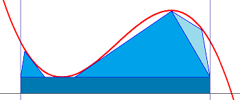
We still teach integration at school basically by this concept, just a bit more structured. We divide the distance between our integration limits into sections of equal width and height being the function value at this point and add all areas. If we choose widths that get smaller and smaller and thus get more and more rectangles then our finite sum turns into an infinite series of converging rectangular areas to which we can assign a value, the questioned integral.

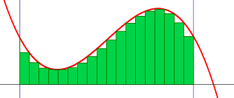
We now call it Riemann or Darboux integration but the idea is from Archimedes.
\begin{align*}
\int_0^1 x\,dx&=\lim_{m \to \infty}\sum_{n=1}^m \dfrac{1}{m}\cdot \dfrac{n}{m}=\lim_{m \to \infty}\dfrac{1}{m^2} \cdot\dfrac{m(m+1)}{2}=\dfrac{1}{2}
\end{align*}
Archimedes’s numerical algorithm to determine $\pi$ to any chosen level of precision is presumably the oldest known numerical algorithm at all.

Functions

The concepts of variables and functions date back to ancient times. How far back depends on how narrow we set up their definitions. Babylonians and Egyptians used word variables already $4,000$ years ago. The transition from word algebra to symbolic algebra can be observed in Diophantus of Alexandria $2,000$ years ago. Diophantus used symbols for the unknown and their powers as well as for arithmetic operations.

“The first approach to implicit usage of the concept of a function in tabular form (shadow length depending on the time of day, chord lengths depending on the central angle, etc.) can already be seen in antiquity. The first evidence of an explicit definition of a function can be found in Nicholas of Oresme (14th century AC), who graphically represented the dependencies of changing quantities (heat, movement, etc.) using perpendicular lines. At the beginning of the process of developing a rigorous understanding of functions were Descartes and Fermat, who developed the analytical method of introducing functions with the help of the variables recently introduced by Vieta. Functional dependencies should therefore be represented by equations such as $y=x^{2}$. This naive concept of functions was retained in school mathematics until well into the second half of the 20th century. The first description of functions according to this idea comes from Gregory in his book Vera circuli et hyperbolae quadratura, published in 1667. The technical term ‘function’ appears for the first time in 1673 in a manuscript by Leibniz, who also used the terms ‘constant’, ‘variable’, ‘ordinate’, and ‘abscissa’ in his treatise De linea ex lineis numero infinitis ordinatim ductis, 1692. The concept of functions is detached from geometry and transferred to algebra in the correspondence between Leibniz and Johann Bernoulli. Bernoulli presents this development in several contributions at the beginning of the 18th century. Leonhard Euler, a student of Johann Bernoulli, further specified functions in his book Introductio in analysin infinitorum in 1748. We can find two different explanations for a function in Euler: On the one hand, every ‘analytic expression’ in $x$ represents a function, on the other hand, $y(x)$ is defined in the coordinate system by a freehand drawn curve. In 1755 he reformulated these ideas without using the term ‘analytic expression’. He also coined the notation $f(x)$ as early as 1734. Euler distinguishes between unique and ambiguous functions. The inverse of the normal parabola, in which every non-negative real number is assigned both its positive and its negative root, is also permitted as a function according to Euler. For Lagrange, only functions that are defined by power series are permissible, as he states in his Théorie des fonctions analytiques in 1797.” [1]

The quotation summarizes the beginning of the concept of functions in the late 17th and entire 18th century. It gives us a brief impression of one of the most fruitful centuries of mathematics. A more elaborate history of calculus can be found e.g. in Dieudonné [2]. The ideas from Newton and Leibniz are barely a century old and here we are: Lagrange uses power series for the first time to define functions,
$$
f(x)=\sum_{n=0}^\infty a_n(x-p)^n .
$$
If we can approximate single numbers by, for example, a geometric series, why not approximate entire functions by series, too? The problem is that we only want to use one series for all function values, i.e. one set of coefficients $a_n$ for any allowed value of $x.$ We do this with polynomials and polynomials are specific power series, namely those with almost all $a_n=0$. So there are examples. But it is hard to imagine a representation by power series for a function like
$$
f(x)=\begin{cases} \phantom{-}1&\text{ if }x\in \mathbb{Q}\\-1&\text{ if }x\not\in\mathbb{Q}\;.\end{cases}
$$
This wouldn’t be a function in Lagrange’s sense. Let’s see how far we get with smooth functions, i.e. infinitely often differentiable functions. We get by the fundamental theorem of calculus, continued integration by parts, and the mean value theorem of integration for some $\xi$
\begin{align*}
f(x)&= f(p)+ \int_p^x f'(t)\,dt = f(p)-\int_p^x f'(t)(x-t)’\,dt\\
&=f(p)+f'(p)(x-p) +\int_p^x f^{”}(t)(x-t)\,dt\\
&=f(p)+f'(p)(x-p) + \frac{1}{2}f^{”}(p)(x-p)^2 + \frac{1}{2}\int_p^x f^{(3)}(t)(x-t)^2\,dt \\
&\phantom{=}\vdots \\
&= \sum_{n=0}^m \dfrac{f^{(n)}(p)}{n!}\cdot (x-p)^n +\frac{1}{m!}\int_p^x f^{(m+1)}(t)(x-t)^m\,dt \\
&= \sum_{n=0}^m \dfrac{f^{(n)}(p)}{n!}\cdot (x-p)^n +\dfrac{f^{(m+1)}(\xi)}{(m+1)!}\cdot (x-p)^{m+1} \quad\text{(Lagrange)}\\
&\phantom{=}\vdots \\
&=\sum_{n=0}^\infty \dfrac{f^{(n)}(p)}{n!}\cdot (x-p)^n\;.
\end{align*}
This series is called the Taylor series of the smooth function $f$ at developing point $p.$ In the case of $p=0,$ we call it a Maclaurin series. The probably most famous Taylor series is the Maclaurin series
$$
e^x=\sum_{n=0}^\infty \dfrac{x^n}{n!}\;.
$$
The little calculation shows us that there exists one power series for all the function values. Well, not quite. Not all functions and their Taylor series are as nice as the exponential function is, or polynomials are. Differentiation that we widely made use of is a local phenomenon, the linear approximation to the function at a certain point. The function values and all derivatives coincide with the Taylor series if we plug in $x=p.$ However, we cannot expect the same for any value further away from $p.$ Hence, the Taylor series is at prior only a formal series. We do not require convergence. There are Taylor series that converge only at $p$, e.g. the Maclaurin series
$$
1-x^2+2!x^4-3!x^6+4!x^8\mp\ldots
$$
built from
$$
f(x)=\int_0^\infty \dfrac{e^{-t}}{1+x^2t}\;dt
$$
converges only for $x=0,$ and there are converging Taylor series that do not converge to the function they were built from, e.g. the Maclaurin series of
$$
f(x)=\begin{cases}e^{-1/x^2} &{\text{if }}x\neq 0\\0&{\text{if }}x=0\;.\end{cases}
$$
The question about how far we can go away from $p$ such that a power series still converges leads us to the concept of the radius of convergence
\begin{align*}
R&=\sup \left\{ |x-p|\, \left| \,\sum_{n=0}^\infty a_n(x-p)^n\text{ converges }\right. \right\}=\dfrac{1}{\displaystyle{\limsup_{n\to \infty } \sqrt[n]{|a_n|} }}\\&=\lim_{n \to \infty}\left|\dfrac{a_n}{a_{n+1}}\right|\quad \text{if the limit exists.}
\end{align*}
Power series converge for $|x|<R$ per definition but it doesn’t say anything about the boundaries. E.g. the power series
$$
\displaystyle{P(\alpha)=\sum_{n=1}^\infty \dfrac{x^n}{n^\alpha}}\quad\text{ with } \alpha\in \{0,1,2\}
$$
all have a radius of convergence $R=1,$ i.e. they converge for all $|x|<1,$ but have a different behavior at the boundaries. $P(0)$ does not converge for $|x|=1,$ $P(2)$ converges for both points $x=\pm 1,$ and $P(1)$ converges at $x=-1$ and diverges at $x=1.$ We have seen that a zero radius of convergence $R=0$ is possible, too.

The relationship between functions and power series becomes really interesting in complex analysis where strange things happen. The simple fact that the complex numbers are more than a two-dimensional real vector space because $\mathrm{i}^2=-1$ allows us to connect one dimension with the other has astonishing consequences.

A complex function $f$ is called analytic in a neighborhood $D$ of a point $z=p$ if it can be developed into a power series on $D$, its Taylor series. Analytic functions are holomorphic, which means they are complex differentiable, and vice versa. The differentiability of a complex function implies already that it is infinitely often differentiable, i.e. it is smooth. The function values of a holomorphic function in the interior of $D$ can be determined by its function values on the border of $D$ by Cauchy’s integral formula
$$ f(z)=\dfrac{1}{2\pi i} \oint_{\partial D} \dfrac{f(\zeta)}{\zeta – z}\,d\zeta\,.$$
All these apparently different properties (analytic, holomorphic, smooth, integral formula) are actually all equivalent for complex functions. Everywhere holomorphic functions, so-called entire functions, that are bounded are even constant by the theorem of Liouville,
$$
\left|f'(z)\right|=\left|\dfrac{1}{2\pi i} \oint_{\partial D} \dfrac{f(\zeta)}{(\zeta – z)^2}\,d\zeta \right|\leq \dfrac{1}{2\pi}\cdot 2\pi r \cdot \dfrac{C}{r^2}\stackrel{r\to \infty }{\longrightarrow }0
$$
and functions whose first derivative is zero are constant. Let us now perform the trick with the geometric series
\begin{align*}
\dfrac{1}{\zeta – z}&=\dfrac{1}{(\zeta -z_0)-(z-z_0)}=\dfrac{1}{\zeta -z_0}\cdot \dfrac{1}{1-\dfrac{z-z_0}{\zeta-z_0}}=\dfrac{1}{\zeta -z_0}\cdot \sum_{n=0}^\infty \left(\dfrac{z-z_0}{\zeta-z_0}\right)^n
\end{align*}
and obtain
\begin{align*}
f(z)=\dfrac{1}{2\pi i}\oint_\gamma \dfrac{f(\zeta)}{\zeta – z}\,d\zeta= \sum_{n=0}^\infty \underbrace{\left(\dfrac{1}{2\pi i} \oint_\gamma \dfrac{f(\zeta)}{(\zeta-z_0)^{n+1}}\,d\zeta \right)}_{=:a_n}\cdot (z-z_0)^n.
\end{align*}
This demonstrates the close relationship between complex differentiability and power series.

Convergence

A series can be assigned a limit to if it converges, i.e. the sequence of its partial sums converges. We have seen an example of a series of rational numbers that converge to $\pi/4$ which is no longer rational. Convergence implies the existence of the limit. We will now assume the completeness of the topological spaces which we pick the series members from, e.g. real or complex numbers, Hilbert spaces, Banach spaces, or p-adic numbers, in order to guarantee the existence of limits so that we do not have to deal with such subtleties of series that intuitively converge but their limits are out of reach.

Completeness has another big advantage. It is equivalent to the fact that a sequence converges to a limit if and only if it is a Cauchy sequence, which means that its sequence members get closer and closer the higher the index is, i.e. in our case of a sequence of partial sums
$$
\exists\,L\, : \,\sum_{n=1}^\infty a_n=L\; \Longleftrightarrow \;
\forall\, \varepsilon>0 \quad \exists\, N_\varepsilon \in\mathbb{N} \quad \forall\, m,n \ge N_\varepsilon \, : \, \left|\sum_{k=n}^m a_k \right|<\varepsilon \,.
$$
This is the first of two main criteria for convergence. It is called the Cauchy criterion. Instead of proving
$$
\forall\, \varepsilon>0 \quad \exists\, N_\varepsilon \in\mathbb{N} \quad \forall\, m \ge N_\varepsilon \, : \, \left|\sum_{n=1}^m a_n -L\right|< \varepsilon
$$
that would require the knowledge of a limit $L$ in advance, the Cauchy criterion does not. It also means that $|a_n|<\varepsilon$ for large indexes, i.e. that $(a_n)_{n\in \mathbb{N}}$ converges necessarily toward zero if the series converges
$$
\exists\,L\, : \,\sum_{n=1}^\infty a_n=L\; \Longrightarrow \;\lim_{n \to \infty}a_n=0\,.
$$
We do not call this a criterion of convergence since it is only a necessity, and not sufficient. The standard counterexample is the harmonic series
$$
\sum_{n=1}^\infty \dfrac{1}{n}
$$
that diverges although its members build a sequence converging to zero as Nicole Oresme has shown in the $14$-th century for the first time:
$$
\begin{matrix}S_{m}&= 1 + 1/2&+&(1/3+1/4)&+&(1/5+1/6+1/7+1/8)&+ \cdots + 1/m\\&\geq 1 + 1/2&+&(1/4+1/4)&+&(1/8+1/8+1/8+1/8)&+ \cdots + 1/m\\&= 1 + 1/2&+&1/2&+&1/2&\ + \cdots + 1/m.\end{matrix}
$$
The main arguments to prove the convergence (or divergence) of a series of numbers are comparisons with series we already know that they converge (or diverge). The problem is that if we bound a series from one side, it is still possible that it escapes us at the other. Hence we need a criterion that works on both sides.
\begin{align*}
|a_n|<b_n \text{ for almost all }n\in \mathbb{N} \;\&\; \sum_{n=1}^\infty b_n \text{ converges } &\Longrightarrow \sum_{n=1}^\infty a_n \text{ converges }\\
|a_n|<b_n \text{ for almost all }n\in \mathbb{N} \;\&\; \sum_{n=1}^\infty a_n \text{ diverges } &\Longrightarrow \sum_{n=1}^\infty b_n \text{ diverges }
\end{align*}This is called the comparison test and is the other major criterion of convergence, proven with the former one
$$
\left|\sum_{k=n}^m a_k\right|\leq \sum_{k=n}^m |a_k|\leq \sum_{k=n}^m b_k <\varepsilon .
$$
The almost all part means up to finitely many. Of course, we can always manipulate finite many $a_n$ and correct the assigned value of the series by the finite sum over those members accordingly without changing the behavior of convergence. A common notation is $|a_n|\leq_{a.a.}b_n.$ We say that the series $\sum_{n=1}^\infty a_n$ converges absolutely since even the series of absolute values $\sum_{n=1}^\infty |a_n|$ converges.

Absolute converging series can be arbitrarily rearranged without changing the limit. This is not the case for converging series in general. E.g. the alternating harmonic series converges …
\begin{align*}
\log(x+1)&=\int_0^x\dfrac{dt}{1+t}\stackrel{\text{Maclaurin}}{=}\int_0^x\sum_{n=0}^\infty \dfrac{\left.\left((1+t)^{-1}\right)^{(n)}\right|_{t=0}}{n!}(t-0)^n\,dt\\
&=\int_0^x\sum_{n=0}^\infty (-1)^{n}\,t^n\,dt =\sum_{n=0}^\infty\int_0^x (-1)^{n}\,t^n\,dt=\sum_{n=1}^\infty \dfrac{(-1)^{n+1}}{n}\,x^n,
\end{align*}
hence
$$
\sum_{n=1}^\infty \dfrac{(-1)^{n+1}}{n}=1-\dfrac{1}{2}+\dfrac{1}{3}-\dfrac{1}{4}\pm\ldots=\log 2
$$
… but by the Riemann series theorem, there exists a rearrangement of indexes $n\mapsto \sigma(n)$ for every real number $c$ such that
$$
\sum_{n=1}^\infty \dfrac{(-1)^{\sigma (n)+1}}{\sigma (n)}=c,
$$
and even divergence can be achieved. E.g., let’s consider the rearrangement
\begin{align*}
\sum_{n=1}^\infty &\left(\dfrac{1}{2n-1}-\dfrac{1}{2(2n-1)}-\dfrac{1}{4n}\right)=\sum_{n=1}^\infty \left(\dfrac{2-1}{2(2n-1)}-\dfrac{1}{2\cdot 2n}\right)\\
&=\dfrac{1}{2}\sum_{n=1}^\infty \left(\dfrac{(-1)^{2n}}{2n-1}+\dfrac{(-1)^{2n+1}}{2n}\right)=\dfrac{1}{2}\sum_{n=1}^\infty \dfrac{(-1)^{n+1}}{n}=\dfrac{1}{2}\log 2
\end{align*}
where we end up with the value $\log\sqrt{2}$ instead of $\log 2$ by exactly the same members of the alternating series only in another order.

We get a few new convergence criteria resulting from the comparison test. There is the ratio test
\begin{align*}
\left|\dfrac{a_{n+1}}{a_n}\right|\leq_{a.a.} q<1 &\Longrightarrow \sum_{n=1}^\infty |a_n|\leq |a_1|\sum_{n=0}^\infty q^n= \dfrac{|a_1|}{1-q}\text{ (absolute convergence)}\\
\left|\dfrac{a_{n+1}}{a_n}\right|\geq_{a.a.} 1&\Longrightarrow \sum_{n=1}^\infty a_n\text{ diverges,}
\end{align*}
the root test
\begin{align*}
\limsup_{n\to\infty }\sqrt[n]{|a_n|}=C<1&\Longrightarrow \sqrt[n]{|a_n|}\leq_{a.a.}C+\dfrac{1-C}{2}=\dfrac{C+1}{2}=:q<1 \\
&\Longrightarrow \sum_{n=1}^\infty |a_n|\leq |a_1|\sum_{n=0}^\infty q^n= \dfrac{|a_1|}{1-q}\text{ (absolute convergence)}\\
\sqrt[n]{|a_n|}\geq_{a.a.} 1 &\Longrightarrow \sum_{n=1}^\infty a_n\text{ diverges,}
\end{align*}
and the integral test for monotone decreasing, non-negative, and integrable functions $f$ on $[p,\infty )$ for some $p\in \mathbb{Z}$
$$
\int_p^\infty f(x)\,dx <\infty \Longleftrightarrow \sum_{n=p}^\infty f(n) \text{ converges.}
$$
The integral test is proven by the comparison test on the intervals between two consecutive integers. In the case of convergence, we have
$$
\sum_{n=p+1}^\infty f(n)\leq \int_p^\infty f(x)\,dx \leq \sum_{n=p}^\infty f(n).
$$
A bit trickier but still by comparisons, is the Leibniz criterion for alternating series, i.e. series that change the sign with every member
$$
a_1 \ge a_2\ge \ldots\ge a_n\ge \ldots\ge 0\;\&\;\lim_{n \to \infty}a_n=0\Longrightarrow \sum_{n=1}^\infty (-1)^na_n\text{ converges.}
$$
The idea is to consider the subsequences of partial sums built from only odd and only even indexes which both converge since they are monotone decreasing, resp. increasing and bounded, and proving that both limits coincide.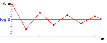

In the end, we have the Cauchy criterion and completeness that guarantee us the existence of a limit and the necessary condition that the series members build a sequence converging to zero, the comparison test and its corollaries, and the Leibniz criterion to prove convergence or divergence of a series.

Domains of Series

Let $R$ be a unitary, commutative ring and
$$
\sum_{n=0}^\infty a_n\, , \,\sum_{n=0}^\infty b_n\ \ (a_n,b_n \in R).
$$
Then we can add, and multiply these series by the rules
\begin{align*}
\sum_{n=0}^\infty a_n + \sum_{n=0}^\infty b_n &= \sum_{n=0}^\infty (a_n+b_n),\\
\sum_{n=0}^\infty a_n \;\cdot\, \sum_{n=0}^\infty b_n &= \sum_{n=0}^\infty \left(\sum_{k=0}^na_kb_{n-k}\right)= \sum_{n=0}^\infty \left(\sum_{p+q=n}a_p b_q\right).
\end{align*}
The resulting series are formal sums as long as we do not specify the ring and define what infinity means. Sums and products of smooth, i.e. analytical real or complex functions are smooth again, so it makes sense that summation and multiplication do not destroy this property. The finite case – polynomials – is also automatically covered by these rules. The multiplication rule is in fact the special case of a (discrete) convolution which is called the Cauchy product or Cauchy product formula in the world of series. If $R$ is a vector space, i.e. an algebra, we can extend the scalar multiplication to
$$
\lambda \cdot \sum_{n=0}^\infty a_n = \sum_{n=0}^\infty \lambda \cdot a_n,
$$
and obtain a vector space and an associative algebra of series.

Let us continue with a non-associative example. One of the fundamental concepts in physics is the correspondence between the symmetry groups of equations and their first order, linear approximations, their (left-invariant, tangent) vector fields; the correspondence between Lie groups $G$, i.e. groups whose group multiplication and inversion are analytical functions and their Lie algebras $\mathfrak{g}$, their tangent space at the identity element. It culminates in the equation [7]
$$
\operatorname{Ad}\exp(X)=\exp(\operatorname{ad}X)\quad (*)
$$
where $X\in \mathfrak{g}$ is a vector field, and $\operatorname{Ad}$, and $\operatorname{ad}$ are the adjoint representations of the Lie group and its Lie algebra, resp. The Lie algebra is non-associative, but the equation itself takes place in an algebraic, and associative matrix group and the exponential function is the series we already know
\begin{align*}
\exp\left(\begin{pmatrix}1&\lambda \\0&-1\end{pmatrix}\right) &=\sum_{n=0}^\infty \dfrac{1}{n!} \begin{pmatrix}1&\lambda \\0&-1\end{pmatrix}^n\\
&=\sum_{n=0}^\infty \dfrac{1}{(2n)!} \begin{pmatrix}1&0\\0&1\end{pmatrix}+\sum_{n=0}^\infty \dfrac{1}{(2n+1)!}\begin{pmatrix}1&\lambda \\0&-1\end{pmatrix}\\
&=\begin{pmatrix}\cosh(1)&0\\0&\cosh(1)\end{pmatrix}+\begin{pmatrix}\sinh(1)&\lambda \sinh(1)\\0&-\sinh(1)\end{pmatrix}\\
&=\begin{pmatrix}\mathrm{e}&\lambda \sinh(1)\\0&1/\mathrm{e} \end{pmatrix}
\end{align*}
We note that the condition $\operatorname{trace}(X)=0$ becomes $\operatorname{det}(\exp X)=1$ and $0\in \mathfrak{g}$ becomes $1\in G$ by exponentiation, the point where the group and its tangent space coincide.

The exponentiation of matrices makes the equation $(*)$ non-trivial and requires precise considerations of infinities (and infinitesimals) if the matrix represents a vector field and exponentiation means solving a differential equation along a flow through it. The example here should only demonstrate that even matrices occur as series members.

 

We remain on the formal side of series manipulations if we consider formal power series over $R$. That is we have the series
$$
\sum_{n=0}^\infty a_nX^n\, , \,\sum_{n=0}^\infty b_nX^n\ \ (a_n,b_n \in R)
$$
in which $X$ is an indeterminate over $R,$ a variable. The rules for addition and multiplication are the same, we only replace $a_n$ by $a_nX^n$ and $b_n$ by $b_nX^n$. The ring of formal power series is denoted by $R[[X]].$ If we allow finitely many negative indices, i.e.
$$
\sum_{n=m}^\infty a_nX^n\ \ (a_n \in R\ ,\ m\in\mathbb{Z})
$$
then we get the ring of Laurent polynomials, denoted by $R(\!(X)\!).$ It is the localization of $R[[X]]$ at the point $X.$ This is the official reading for: we allow $X$ to have an inverse. In case $R=\mathbb{F}$ is a field, we get algebras over $\mathbb{F},$ embeddings
$$
\begin{array}{ccc}\mathbb{F}[X]&\rightarrowtail &\mathbb{F}[[X]]\\ \downarrow &&\downarrow \\\mathbb{F}(X)&\rightarrowtail &\mathbb{F}(\!(X)\!)\end{array}
$$
and find ourselves in the middle of abstract algebra: we have a formal differentiation, we can identify our series with infinite sequences, we have a metric, and therewith a topology, completions, etc. It is the effort to take as many properties from calculus as possible to abstract algebra.

 

We finally have a closer look at our number systems. The usual hierarchy from the semigroup of natural numbers to quaternions and octonions is
\begin{align*}
\mathbb{N} \;\subset\;\mathbb{N}_0 \;\subset\; \mathbb{Z} \;\subset\; \mathbb{Q} \;\subset\; \mathbb{R} \;\subset\; \mathbb{C} \;\subset\; \mathbb{H}\;\subset\; \mathbb{O}
\end{align*}
and we use occasionally finite systems $\mathbb{Z}_n,$ e.g. $\mathbb{Z}_2$ on light switches and in computers, or $\mathbb{Z}_{12}$ for those of us who still have an analog wrist watch. The step $\mathbb{Q}\subset \mathbb{R}$ was of particular importance for series as it provided the existence of limits. The real numbers are the topological completion of the rational numbers, the complex numbers are the algebraic completion (algebraic closure) of the real numbers.

In $1897,$ Kurt Hensel came up with a different idea to complete the rational numbers. We can write every real number as a series
$$
\pm\sum_{n=-\infty }^m a_np^n \quad (0\le a_n <p).
$$
for some natural number $p.$ We do this with decimal numbers where the base is $10,$ the Babylonians used $60,$ digital (binary) numbers have the base $2.$ We can do the same with any number $p.$ These series converge according to the absolute value. Hensel’s idea was to turn it upside down. Let therefore be $p$ a prime number, $a=p^r \cdot x$ and $b = p^s \cdot y$ with $p \nmid xy.$ Then
$$
\left|\dfrac{a}{b}\right|_p = \begin{cases}  p^{-r+s} &\text{ if } a \neq 0\\ 0&\text{ if }a=0\end{cases}
$$
defines a valuation and a distance by
$$
d(a,b)=|a-b|_p\;.
$$
The series
$$
\pm\sum_{n=m}^\infty a_np^n \quad (0\le a_n <p\, , \,m\in \mathbb{Z})
$$
now converge by this new definition of a distance, and every rational number can be written this way, e.g. [8]. With the distance comes the opportunity of a completion (converging Cauchy sequences), and by the convergence of the above series, we get the $p$-adic numbers
$$
\mathbb{Q}\subset \mathbb{Q}_p=\left\{\left. \pm\sum_{n=m}^\infty a_np^n \; \right| 0\le a_n <p\, , \,m\in \mathbb{Z}\;\right\}.
$$

Sources