An Overview of Complex Differentiation and Integration

Abstract

I want to shed some light on complex analysis without getting all the technical details in the way which are necessary for the precise treatments that can be found in many excellent standard textbooks.

Analysis is about differentiation. Hence, complex differentiation will be my starting point. It is simultaneously my finish line because its inverse, the complex integration, is closely interwoven with complex differentiation. By the lack of details, I mean that I will sometimes assume a disc if a star-shaped region or a simply connected open set would be sufficient; or assume a differentiable function if differentiability up to finitely many points would already be sufficient. Also, the sometimes necessary techniques of gluing triangles for an integration path, or the epsilontic within a region will be omitted.

The statements listed as theorems, however, will be precise. Some of them might sometimes allow a wider range of validity, i.e. more generality. Nevertheless, the reader will find the basic ideas, definitions, tricks, and theorems of the residue calculus; and if nothing else, see where all the $\pi$’s in integral formulas come from.

Complex Differentiation

A function $f:U\rightarrow V$ is differentiable at $x_0$ if there is a linear approximation $D_{x_0}f=(Df)_{x_0}$, such that (Karl T.W. Weierstraß)
\begin{equation*}
f(x_0+v)=f(x_{0})+(D_{x_0}f)\cdot v+r(v)
\end{equation*}
where the error function $r$ has the property, that it converges faster to zero than linear in any direction $v$, which means
$$\lim_{v \rightarrow 0}\frac{r(v)}{v}=0.$$
If we rearrange this formula, then
\begin{align*}
D_{x_0}f&= \lim_{v\to 0}D_{x_0}f = \lim_{v\to 0}\left( \dfrac{f(x_0+v)-f(x_0)}{v}-\dfrac{r(v)}{v}\right)=\lim_{v\to 0} \dfrac{f(x_0+v)-f(x_0)}{v}
\end{align*}
reveals the formula that is commonly used to define a derivative. It also shows that
$$
D_{x_0}f=(Df)_{x_0}=\left. \dfrac{df}{dx}\right|_{x_0}=f'(x_0)
$$
If $f$ is a function of a one-dimensional range, then the direction $v$ can only be a one-dimensional vector and we assume $v=1$ when we write
$$f'(x_0)=f'(x_0)\cdot 1= D_{x_0}f\cdot v.$$
The beauty of Weierstraß’s formula lies in the fact that it carries all the important properties of a derivative:

• locality:
  Weierstraß’s formula requires validity in a region of $x_0.$
• linear operator and Leibniz rule:
  $D_{x_0}$ is a derivation, i.e. $D_{x_0}(\alpha\cdot f+\beta\cdot g)=\alpha\cdot D_{x_0}(f) +\beta\cdot D_{x_0}(g)$ and $D_{x_0}(f\cdot g)=D_{x_0}(f)g(x_0)+f(x_0)D_{x_0}(g).$
• linearity:
  $D_{x_0}f$ is a linear function, i.e. $D_{x_0}f(\alpha v+\beta w)=\alpha D_{x_0}f(v)+\beta D_{x_0}f(w).$
• directionality, slope:
  A derivative $(D_{x_0}f) v$ is directional, namely the slope in direction $v.$
• approximation:
  $r(v)=o(v).$

By allowing all parts $x_0,f,v,r,D,D_{x_0},D_{x_0}f, D_{*}f$ in Weierstraß’s formula to be variables of an operator in its most general meaning, we immediately open the door to fiber bundles, global and local sections, differential forms and tangent- as well as cotangent bundles. Also note that we did not distinguish between real and complex functions, yet. This generality shall be our starting point.

Every complex linear function $\varphi : \mathbb{C}\rightarrow \mathbb{C}$ is a real linear function, too, and can be written as
\begin{align*}
\varphi(x+iy)&=\underbrace{\begin{pmatrix}\varphi_{11}&\varphi_{12}\\\varphi_{21}&\varphi_{22}\end{pmatrix}}_{\in \mathbb{M}(2,\mathbb{R})}(x+iy)=(\varphi_{11}(x)+\varphi_{12}(y))+i(\varphi_{21}(x)+\varphi_{22}(y))
\end{align*}
$\mathbb{C}$-linearity means that
$$
(a+ib)\varphi(x+iy)=\varphi((ax-by)+i(bx+ay))
$$
and thus
\begin{align*}
(a+ib)&\cdot (\varphi_{11}(x)+\varphi_{12}(y))+i(\varphi_{21}(x)+\varphi_{22}(y))\\
&=(\varphi_{11}(ax)+\varphi_{12}(ay)-\varphi_{21}(bx)-\varphi_{22}(by))\\
&\phantom{=}+i(\varphi_{11}(bx)+\varphi_{12}(by)+\varphi_{21}(ax)+\varphi_{22}(ay))\\
&=(\varphi_{11}(ax)-\varphi_{11}(by)+\varphi_{12}(bx)+\varphi_{12}(ay))\\
&\phantom{=}+i(\varphi_{21}(ax)-\varphi_{21}(by)+\varphi_{22}(bx)+\varphi_{22}(ay))
\end{align*}
Comparing both sides results in
\begin{align*}
\varphi_{11}=\varphi_{22}\, &\text{ and } \,\varphi_{21}+\varphi_{12}=0\quad (*)
\end{align*}
We know that $D_{z_0}$ is a $\mathbb{C}$-linear operator, and $D_{z_0}f$ is a $\mathbb{C}$-linear function. If we write $f=u+iv$ then
$$
D_{z_0}f=D_{z_0}u+iD_{z_0}v=\left( \left.\dfrac{\partial u}{\partial x}\right|_{z_0}dx+\left.\dfrac{\partial u}{\partial y}\right|_{z_0}dy\right)+i\left(\left.\dfrac{\partial v}{\partial x}\right|_{z_0}dx+\left.\dfrac{\partial v}{\partial y}\right|_{z_0}dy\right)
$$
and our condition $(*)$ of $\mathbb{C}$-linearity becomes
$$
\left. \dfrac{\partial u}{\partial x }\right|_{z_0} = \left. \dfrac{\partial v}{\partial y}\right|_{z_0}\text{ and }\left. \dfrac{\partial u}{\partial y}\right|_{z_0}+\left. \dfrac{\partial v}{\partial x}\right|_{z_0}=0\,,
$$
the Cauchy-Riemann equations. This means that complex differentiability is real differentiability plus the Cauchy-Riemann equations. This is the main difference why complex analysis is more than $\mathbb{R}^2$ analysis, complex linearity.

Holomorphic Functions

We see by induction that skew-symmetric matrices with a constant diagonal (spiral symmetry) keep their structure if we multiply them by themselves
\begin{align*}
\begin{pmatrix}a&b\\-b&a\end{pmatrix}^{n+1}&=\begin{pmatrix}c&d\\-d&c\end{pmatrix}\cdot \begin{pmatrix}a&b\\-b&a\end{pmatrix}=\begin{pmatrix}ca-db&cb+da\\-da-cb&-db+ca\end{pmatrix}
\end{align*}
That means the Cauchy-Riemann property is invariant under exponentiation
$$
\begin{pmatrix}\dfrac{\partial u}{\partial x}&\dfrac{\partial u}{\partial y}\\[16pt] \dfrac{\partial v}{\partial x}&\dfrac{\partial v}{\partial y}\end{pmatrix}^n=\begin{pmatrix}\dfrac{\partial u}{\partial x}&\dfrac{\partial u}{\partial y}\\[16pt] -\dfrac{\partial u}{\partial y}&\dfrac{\partial u}{\partial x}\end{pmatrix}^n=
\begin{pmatrix}
p\left(\dfrac{\partial u}{\partial x}\, , \,\dfrac{\partial u}{\partial y}\right) & q\left(\dfrac{\partial u}{\partial x}\, , \,\dfrac{\partial u}{\partial y}\right) \\[16pt]
-q\left(\dfrac{\partial u}{\partial x}\, , \,\dfrac{\partial u}{\partial y}\right) & p\left(\dfrac{\partial u}{\partial x}\, , \,\dfrac{\partial u}{\partial y}\right)
\end{pmatrix}
$$
for some real polynomials $p(X,Y,n),q(X,Y,n)\in \mathbb{R}[X,Y].$

Definition: A complex function $f:U\rightarrow V$ is holomorphic if it is complex differentiable in a non-empty, open, and connected set $U$, i.e. in a region. $f$ is called meromorphic if it is holomorphic up to a set of isolated points, its poles. If $f$ is holomorphic on the entire complex plane, then it is called an entire function. A real, or complex function is analytic at a point $z_0\in U$, if there is a power series that converges to the function value in an open neighborhood of $z_0$
$$
f(z)=\sum_{n=0}^\infty a_n(z-z_0)^n.
$$

Theorem: The following statements for $f=u+iv\, : \,U\rightarrow V$ are equivalent:

1. $f$ is complex differentiable in a region $U,$ $f\in C^1(U).$
2. $f$ is arbitrary often complex differentiable in a region $U,$ $f\in C^\infty (U).$
3. $f$ is holomorphic on $U,$ $f\in \mathcal{O}(U).$
4. The real and imaginary parts of $f$ are continuously real differentiable and fulfill the Cauchy-Riemann partial differential equations (CR).
5. $f$ is analytic on $U.$
6. $f$ is real differentiable and ${\displaystyle {\tfrac{\partial f}{\partial {\bar {z}}}}:={\tfrac{1}{2}} \left({\tfrac{\partial }{\partial x}} + i {\tfrac{\partial }{\partial y}}\right)}(f) =0.$

Complex Line Integrals

We have seen that the definition of complex differentiation doesn’t require a change of real differentiation, just the reminder that the field $\mathbb{C}$ which replaces the field $\mathbb{R}$ may not be confused with the real vector space $\mathbb{R}^2.$ We are used to imagining complex numbers as points in the complex plane, but the complex numbers are not a real plane, they are a one-dimensional complex vector space over themselves.

The inverse operation is integration. And real integration is the calculation of an oriented volume, an area (volume of the area under the function graph) in the case of a function $g:\mathbb{R}\rightarrow \mathbb{R}.$ Oriented means that we distinguish the areas above the $x$-axis from the areas below the $x$-axis, as well as the integration path from $x=a$ to $x=b$ from the integration path from $x=b$ to $x=a.$ If the function itself is a straight, say $g(x)=r,$ then the area is that of a single rectangle
$$
\int_a^b g(x)\,dx=\int_a^b r\,dx=[rx]_a^b=rb-ra=r\cdot (b-a).
$$
If we proceed as above and only substitute the real numbers with complex numbers, then we get
\begin{align*}
\int_{a+ic}^{b+id} g(x)\,dx&=\int_{a+ic}^{b+id} (r+is)\,dz=[(r+is)z]_{a+ic}^{b+id}\\
&=(r(b-a)-s(d-c))+i(r(d-c)+s(b-a))\\
&=\int_a^b r\,dz +\int_{ic}^{id}(is)\,dz+ \int_{ic}^{id}r\,dz+\int_{a}^b (is)\,dz \,.
\end{align*}
Only the number of distinguishable orientations increases because $i \cdot i = -1$ creates another negative area and imaginary volumes are allowed. This means we have to investigate the integration path more carefully than just from left to right or from right to left as we did in real integration if we want to understand a complex volume built by complex lengths. Fortunately, the integral itself cares about all orientations as long as we don’t make a sign error, and as long as we are not interested in an actual geometric volume, that had to be positive and real.

To begin with, we define the obvious integral
$$
\int_a^b f(t)\,dt := \int_a^b u(t)\,dt +i\int_a^b v(t)\,dt
$$
for (piecewise) continuous functions $f=u+iv : \mathbb{R}\supset [a,b] \rightarrow \mathbb{C}.$

We also use this for the definition of the complex line integral $\displaystyle{\int_{z_1}^{z_2}f(z) \,dz}$ where we integrate along a (real) parameterized path $\gamma: [a,b] \longrightarrow G\subseteq \mathbb{C}$ from $\gamma (a)=z_1\in G,\gamma (b)=z_2\in G$ for a complex function $f: G\longrightarrow \mathbb{C}$ defined on a region $G\subseteq \mathbb{C}$
\begin{align*}
\int_\gamma f(z)\,dz &=…\text{ (substitution }z=\gamma(t)\, , \,dz=\gamma’\,dt) \\
…&=\int_a^b (f\circ \gamma )(t)\cdot \gamma’\,dt =\int_a^b f(\gamma (t))\cdot \gamma'(t)\,dt
\end{align*}
The complex line integral depends on a priori on the integration path! This can easily be shown for $f(z)=\bar{z}.$ However, if $f$ is holomorphic, then its line integrals are path independent.

 

Cauchy’s Integral Theorem: If $f:G\longrightarrow \mathbb{C}$ is a continuous complex function then $f$ has an anti-derivative on $G$ if and only if $\displaystyle{\oint_\gamma f(z)\,dz=0}$ for any closed integration path $\gamma$ in $G$, $\gamma(a)=z_0=\gamma(b).$

Both is true for a star-shaped region $G,$ e.g. a convex region, and a holomorphic function $f.$

 

Example: Consider the border $\gamma(t)=z_0+re^{i t}\, , \,0\leq t\leq 2\pi$ of the disc $G=D_r(z_0)$ around a central point $z_0.$ Then
\begin{align*}
\oint_\gamma \dfrac{1}{z-z_0}\,dz&=\int_0^{2\pi}\dfrac{1}{re^{it}} \cdot ire^{it} \,dt=i\cdot \int_0^{2\pi}dt=2\pi i\\
\oint_\gamma \left(z-z_0\right)^p\,dz&\stackrel{(p\neq -1)}{=}\int_0^{2\pi} r^p e^{i p t} \cdot ire^{it}\,dt=ir^{p+1}\int_0^{2\pi} e^{i(p+1)t}\,dt\\
&=ir^{p+1}\left[\dfrac{e^{i(p+1)t}}{i(p+1)}\right]_0^{2\pi}=\dfrac{r^{p+1}}{p+1}(e^{2(p+1)\pi i t}-e^0)=0\,.
\end{align*}
Hence, we get the important formula
$$
\oint_\gamma \left(z-z_0\right)^p\,dz=\begin{cases}
2\pi i & \text{ if } p = -1 \\
0 & \text{ if } p\neq -1 \,.
\end{cases}
$$

Corollary: If $D\subset \mathbb{C}$ is a disc, and $z\in \mathbb{C} \backslash \partial D$ then
$$
\oint_{\partial D} \,\dfrac{d\zeta}{\zeta -z}=\begin{cases}
2\pi i & \text{ if } z\in D \\
0 & \text{ else } \,.
\end{cases}
$$

Complex Integration

If $f:G\rightarrow \mathbb{C}$ is holomorphic, then
$$
f(\zeta)=f(z)+\underbrace{\left( (D_{z}f)+\underbrace{\dfrac{r(\zeta-z)}{\zeta-z}}_{\stackrel{\zeta \to z}{\longrightarrow }\;\;0} \right)}_{=:\Delta_z(\zeta)}\cdot (\zeta-z)
$$
with an everywhere continuous and besides $z$ even holomorphic function $\Delta_z.$ Thus
\begin{align*}
0&=\oint_{\partial D}\Delta(\zeta)\,d\zeta =\oint_{\partial D}\dfrac{f(\zeta)-f(z)}{\zeta -z}\,d\zeta \\
&=\oint_{\partial D}\dfrac{f(\zeta)}{\zeta -z}\,d\zeta – f(z) \oint_{\partial D}\dfrac{1}{\zeta -z}\,d\zeta =\oint_{\partial D}\dfrac{f(\zeta)}{\zeta -z}\,d\zeta – f(z)\cdot 2\pi i
\end{align*}
and
$$
f(z)=\dfrac{1}{2\pi i}\oint_{\partial D}\dfrac{f(\zeta)}{\zeta -z}\,d\zeta
$$
We even have

Theorem: The following statements for $f=u+iv\, : \,U\rightarrow V$ are equivalent:

1. $f$ is holomorphic on $U.$
2. $f$ is continuous and its path integral over any closed, contractible path vanishes.
3. The function values of $f$ on the interior of a disc $D\subseteq U$ can be determined by the function values on the border of this disc by Cauchy’s integral formula
   $$ f(z)=\dfrac{1}{2\pi i} \oint_{\partial D} \dfrac{f(\zeta)}{\zeta – z}\,d\zeta\,.$$

Let us now introduce the trick with the geometric series. $f:D\rightarrow \mathbb{C}$ be a continuous function an a compact set $D\, , \, z_0\not\in D$ and $R=\operatorname{dist}(z_0,D).$ Then
\begin{align*}
\dfrac{1}{\zeta – z}&=\dfrac{1}{(\zeta -z_0)-(z-z_0)}=\dfrac{1}{\zeta -z_0}\cdot \dfrac{1}{1-\dfrac{z-z_0}{\zeta-z_0}}=\dfrac{1}{\zeta -z_0}\cdot \sum_{n=0}^\infty \left(\dfrac{z-z_0}{\zeta-z_0}\right)^n
\end{align*}
for $|z-z_0|<R\leq |\zeta-z_0|$ and $z\in D_R(z_0)\, , \,\zeta \in D.$ Since $f$ is bounded on the compact set $D,$ say $0<|f(\zeta)|<C,$ we have
$$
\left| \dfrac{f(\zeta)}{(\zeta-z_0)^{n+1}}\cdot(z-z_0)^n \right|\leq \dfrac{C}{R}\cdot \left(\dfrac{z-z_0}{R}\right)^n
$$
and the series on the right converges for any fixed $z\in D_R(z_0).$ Thus
$$
\dfrac{f(\zeta)}{\zeta – z}=\dfrac{f(\zeta)}{\zeta -z_0}\cdot \sum_{n=0}^\infty \left(\dfrac{z-z_0}{\zeta-z_0}\right)^n=\sum_{n=0}^\infty \dfrac{f(\zeta)}{(\zeta-z_0)^{n+1}}\cdot (z-z_0)^n
$$
converges absolutely and uniformly for a fixed $z$ for $\zeta \in D$ by Weierstraß’s criterion. Finally,
\begin{align*}
f(z)=\dfrac{1}{2\pi i}\oint_\gamma \dfrac{f(\zeta)}{\zeta – z}\,d\zeta= \sum_{n=0}^\infty \underbrace{\left(\dfrac{1}{2\pi i} \oint_\gamma \dfrac{f(\zeta)}{(\zeta-z_0)^{n+1}}\,d\zeta \right)}_{=:a_n}\cdot (z-z_0)^n
\end{align*}
converges absolute and uniformly on the interior of $D_R(z_0)$ versus the everywhere holomorphic, and by construction analytic function
$$
f(z)=\sum_{n=0}^\infty a_n(z-z_0)^n\,.
$$
If we apply this to the border of a disc $\gamma(t)=z_0+re^{it}$ with $0<r<R$ and $0\leq t\leq 2\pi ,$ we get

Cauchy’s Expansion Theorem: Let $f:G\rightarrow \mathbb{C}$ be a complex, holomorphic function on a region $G$ and $z_0\in G.$ Let further be $R$ the maximal radius of an open disc around $z_0$ that fits into $G.$ Then there is a power series
$$
f(z)=\sum_{n=0}^\infty a_n(z-z_0)^n,
$$
that converges for all $0<r<R$ on the disc $D_r(z_0)$ absolutely and uniformly versus $f(z).$ For every such $r$ is
$$
\displaystyle{a_n=\dfrac{1}{2\pi i} \oint_{\partial D_r(z_0)} \dfrac{f(\zeta)}{(\zeta-z_0)^{n+1}}\,d\zeta}
$$
and $f$ is on $G$ arbitrary often complex differentiable.

Residue Theorem

Let us start with Laurent’s decomposition trick for a holomorphic function $f:\mathcal{R}\rightarrow \mathbb{C}$ on a ring $\mathcal{R}=\{z\in \mathbb{C}\,|\,0<r<|z|<R\}.$ There exists a decomposition
$$
f(z)=g(z)+h\left(\dfrac{1}{z}\right)
$$
into holomorphic functions on discs
$$
g:D_R(0)\rightarrow \mathbb{C}\; , \;h:D_{1/r}(0)\rightarrow \mathbb{C}
$$
The decomposition becomes unique if we require $h(0)=0.$ Since holomorphic functions are analytic, we have an expansion into power series
$$
f(z)= \sum_{n=0}^\infty a_nz^n+\sum_{n=0}^\infty b_n\left(\dfrac{1}{z}\right)^n=\sum_{n=-\infty }^\infty c_nz^n
$$
For an expansion at $z_0$ we receive a Laurent series $(r<\rho<R)$
$$
f(z)=\sum_{n=-\infty }^\infty a_n (z-z_0)^n\; , \;a_n=\displaystyle{\dfrac{1}{2\pi i} \oint_{\partial D_\rho(z_0)} \dfrac{f(\zeta)}{(\zeta-z_0)^{n+1}}\,d\zeta}
$$
Note that $r=0,R=\infty ,$ and $r=R$ are possible settings. Those radii can be calculated by the formula of Cauchy-Hadamard
$$
r=\limsup_{n\to \infty } \sqrt[n]{|a_{-n}|}\; , \;R=\dfrac{1}{\displaystyle{\limsup_{n\to \infty } \sqrt[n]{|a_{n}|}}}
$$
Definition: Let $f:G\rightarrow \mathbb{C}$ be a holomorphic function that does not completely vanish on the region $G\subseteq \mathbb{C}.$ The coefficient at $-1$
$$
\operatorname{Res}_{z_0}(f)=a_{-1}=\dfrac{1}{2\pi i} \oint_{\partial D_\rho(z_0)} f(\zeta) \,d\zeta
$$
is called the residue of $f$ at $z_0.$ It is the only coefficient without a $z-z_0$ term in the Laurent series of $f.$

A point $z_0$ is called a zero of order $m$ if there is a holomorphic function $g:D_r(z_0)\rightarrow \mathbb{C}$ such that
$$
f(z)=(z-z_0)^m g(z)\; , \;g(z_0)\neq 0 .
$$
A point $z_0$ is called a pole (isolated singularity) of order $m$ if there is a holomorphic function $g:D_r(z_0)\rightarrow \mathbb{C}$ such that
$$
f(z)=(z-z_0)^{-m}g(z)\; , \;g(z_0)\neq 0 .
$$
A pole is a zero of $1/f.$ The residue of a pole of order $m$ is
$$
\operatorname{Res}_{z_0}(f)= \dfrac{1}{(n-1)!} \lim_{z\to z_0}{\dfrac{d^{n-1}}{dz^{n-1}}} \left((z-z_0)^{n}f(z)\right)
$$
We have seen that surrounding a disc once means $\;\dfrac{1}{2\pi i}\displaystyle{\oint_{\partial D} \,\dfrac{d\zeta}{\zeta -z}}=1.$

If we instead have any closed curve $\gamma$ around $z_0,$ then we define the winding number of $\gamma$ around $z_0$ as
$$
\operatorname{Ind}_\gamma (z_0):=\dfrac{1}{2\pi i}\oint_{\gamma} \,\dfrac{d\zeta}{\zeta -z}.
$$

Residue Theorem: Let $f:G\rightarrow \mathbb{C}$ be a holomorphic function up to finitely many isolated singularities $z_1,\ldots,z_q,$ i.e. $f$ is meromorphic, and $\gamma$ a closed, piecewise smooth curve in the region $G,$ then
$$
\oint_\gamma f(z)\,dz=2\pi i \sum_{k=1}^q \operatorname{Ind}_\gamma (z_k) \operatorname{Res}_{z_k}(f)
$$
Let’s call the set of zeros $Z$ and the set of poles $P$ of a meromorphic function $f,$ and require that our integration path $\gamma$ doesn’t contain any of them. We already have seen that we can write $f(z) =(z-z_0)^{m}g(z) = (z-z_0)^{\operatorname{ord}_{z_0}(f)}$ for any $z_0\in Z\cup P$ of order $|m|.$ Then
$$
\dfrac{f'(z)}{f(z)}=\dfrac{m}{z-z_0}+\dfrac{g'(z)}{g(z)}.
$$
$\dfrac{g'(z)}{g(z)}$ is holomorphic at $z_0$ since $g(z_0)\neq 0.$ The residue of $f’/f$ at $z_0$ equals therefore exactly the order $m$ of the zero or pole $z_0$ of $f$ and
$$
\dfrac{1}{2\pi i}\oint_\gamma \dfrac{f'(z)}{f(z)}\,dz=\sum_{z_0\in Z\cup P} \operatorname{Ind}_\gamma (z_0)\cdot \operatorname{Res}_{z_0}\left(\dfrac{f’}{f}\right) =\sum_{z_0\in Z\cup P} \operatorname{Ind}_\gamma (z_0)\cdot \operatorname{ord}_{z_0}(f)
$$
where
$$
\operatorname{Res}_{z_0}\left(\dfrac{f’}{f}\right) = \operatorname{ord}_{z_0}(f)=
\begin{cases}
k & \text{if } z_0 \in Z \text{ of order k }\\
-k & \text{if } z_0 \in P \text{ of order k }\\
0 & \text{ else }
\end{cases}
$$

Properties of Residues

Cauchy’s integral theorem says that $\operatorname{Res}_{z_0}(f)=0$ for a holomorphic function $f:G\rightarrow \mathbb{C}$ and $z_0\in G.$ Let’s see how residues can be calculated in other cases. Say $z_m$ is a zero of order $m$ and $p_m$ a pole of order $m$ of a meromorphic function $f:G\rightarrow \mathbb{C}.$ Let further be $h:G\rightarrow \mathbb{C}$ holomorphic at those points, and $g$ another meromorphic function. Then $\operatorname{Res}_{z_0}$ is $\mathbb{C}$-linear and

$$
\begin{array}{ll}
\operatorname{Res}_{z_0}(\alpha f+\beta g)=\alpha\operatorname{Res}_{z_0}(f)+\beta\operatorname{Res}_{z_0}(g) &(z_0\in G \, , \,\alpha, \beta \in \mathbb{C}) \\[16pt]
\operatorname{Res}_{z_1}\left(\dfrac{h}{f}\right)=\dfrac{h(z_1)}{f'(z_1)}&
\operatorname{Res}_{z_1}\left(\dfrac{1}{f}\right)=\dfrac{1}{f'(z_1)}\\[16pt]
\operatorname{Res}_{z_m}\left(h\dfrac{f’}{f}\right)=h(z_m)\cdot m&\operatorname{Res}_{z_m}\left(\dfrac{f’}{f}\right)=m\\[16pt]
\operatorname{Res}_{p_1}(h\cdot f)=h(p_1)\cdot \operatorname{Res}_{p_1}(f)&\operatorname{Res}_{p_1}(f)=\displaystyle{\lim_{z \to p_1}((z-p_1)f(z))}\\[16pt]
\operatorname{Res}_{p_m}(f)=\dfrac{1}{(m-1)!}\displaystyle{\lim_{z \to p_m}\dfrac{\partial^{m-1} }{\partial z^{m-1}}\left( (z-p_m)^m f(z) \right)}&\operatorname{Res}_{p_m}\left(\dfrac{f’}{f}\right)=-m\\[16pt]
\operatorname{Res}_{\infty }(f)=\operatorname{Res}_0\left(-\dfrac{1}{z^2}f\left(\dfrac{1}{z}\right)\right)&\operatorname{Res}_{p_m}\left(h\dfrac{f’}{f}\right)=-h(p_m)\cdot m\\[16pt]
\operatorname{Res}_{z_0}(h)=0 & \operatorname{Res}_0\left(\dfrac{1}{z}\right)=1\\[16pt]
\operatorname{Res}_1\left(\dfrac{z}{z^2-1}\right)=\operatorname{Res}_{-1}\left(\dfrac{z}{z^2-1}\right)=\dfrac{1}{2}&\operatorname{Res}_0\left(\dfrac{e^z}{z^m}\right)=\dfrac{1}{(m-1)!}
\end{array}
$$

Real Integration with Residues

Consider a real rational function $f:\mathbb{R}\rightarrow \mathbb{R}$ with $\deg(f)\leq -2$ that has no poles on the real axis.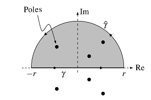

We want to integrate $f$ along the real axis, but take this as a part of the complex plane. Our primary integration path is a composite of the real path $\gamma :[-r,r]\rightarrow [-r,r]\subseteq \mathbb{C}\, , \,\gamma(t)=t$ and the complex path $\tilde{\gamma }:[0,\pi]\rightarrow \mathbb{C}\, , \,\tilde{\gamma }(t)=re^{it}$ in the upper half of the plane where $\mathfrak{Im}(z)\geq 0.$ The residue theorem says

$$
\displaystyle{\oint_{\gamma \oplus \tilde{\gamma }}f(z)\,dz =\int_\gamma f(z)\,dz +\int_{\tilde{\gamma }}f(z)\,dz= 2\pi i\sum_{k=1}^q\operatorname{Res}_{z_k}(f). }
$$
and all poles of $f$ lie within our closed integration path as long as the radius $r$ is large enough. Moreover, for any normed, i.e. the leading coefficient equals $1$, complex polynomial $P(z)$ of degree $n$ there is an $R\in \mathbb{R}^+$ such that for all $z\in \mathbb{C}$ with $|z|\geq R$
$$
\dfrac{1}{2}|z|^n\leq |P(z)|\leq \dfrac{3}{2}|z|^n
$$
which can be proven with the triangle inequalities. We get for our rational function that there is a positive real constant $c\in \mathbb{R}^+$ such that ($L$= length)
$$
\displaystyle{\left|\int_{\tilde{\gamma }}f(z)\,dz\right|\leq L(\gamma )\cdot \max_{|z|=r}|f(z)|\leq \pi r \cdot cr^{-2}=\pi\dfrac{c}{r}\;\stackrel{r\to \infty }{\longrightarrow }\;0}
$$
Hence
\begin{align*}
\int_{-\infty }^\infty f(x)\,dx&= \displaystyle{\lim_{r \to \infty} \int_{-r}^rf(x)\,dx}=\displaystyle{\lim_{r \to \infty} \int_\gamma f(z)\,dz +0}\\
&=\displaystyle{\lim_{r \to \infty} \int_\gamma f(z)\,dz + \lim_{r \to \infty}\int_{\tilde{\gamma }}f(z)\,dz }= 2\pi i\sum_{k=1}^q\operatorname{Res}_{z_k}(f).
\end{align*}

Example: We want to find $\displaystyle{\int_{-\infty }^\infty \dfrac{dx}{(1+x^2)^n}}$ for a positive integer $n\in \mathbb{N}$ which equals $2\pi i \operatorname{Res}_{i}(f)$ for the meromorphic function $$f(x)=\dfrac{1}{(z^2+1)^n}=\dfrac{1}{(z+i)^n(z-i)^n}$$ that has $z=i$ as only pole of order $n$ in the upper half of the complex plane.
\begin{align*}
\operatorname{Res}_{i}\left(\dfrac{1}{(1+z^2)^n}\right)&=\dfrac{1}{(n-1)!}\displaystyle{\;\lim_{z \to i}}\;\dfrac{\partial^{n-1}}{\partial z^{n-1}}\left((z-i)^n\dfrac{1}{(1+z^2)^n}\right)\\
&=\dfrac{1}{(n-1)!}\displaystyle{\;\lim_{z \to i}}\;\dfrac{\partial^{n-1}}{\partial z^{n-1}}(z+i)^{-n}\\
&=\dfrac{1}{(n-1)!}\displaystyle{\;\lim_{z \to i}
(-n)(-n-1)\cdots (-2n+2)(z+i)^{-2n+1}}\\
&=\dfrac{1}{(n-1)!}(-1)^{n-1}\dfrac{(2n-2)!}{(n-1)!}(2i)^{-2n+1}=-\dfrac{i}{2^{-2n+1}}\binom{2n-2}{n-1}
\end{align*}
and
$$
\displaystyle{\int_{-\infty }^\infty \dfrac{dx}{(1+x^2)^n}= \dfrac{\pi}{2^{2n-2}}}\binom{2n-2}{n-1}.
$$
It can be proven by similar methods as above that (cp. Fourier transform)
$$
\int_{-\infty }^\infty f(x)e^{ix}\,dx=2\pi i \sum_{k=1}^q\operatorname{Res}_{z_k}\left(f(z)e^{iz}\right)
$$
for a real rational function $f$ with $\deg(f)\leq -2$ and poles $z_1,\ldots,z_q$ on the strict upper half of the complex plane, i.e. $\mathfrak{Im}(z_k)>0.$

Example:

\begin{align*}
\int_{-\infty }^\infty \dfrac{\cos x}{1+x^2}\,dx&=\mathfrak{Re}\left(\int_{-\infty }^\infty \dfrac{\frac{1}{2}(e^{ix}+e^{-ix})}{1+x^2}\,dx \right)=\mathfrak{Re}\left(\int_{-\infty }^\infty \dfrac{e^{ix}}{1+x^2}\,dx\right)\\
&=\mathfrak{Re}\left(2\pi i \operatorname{Res}_{i}\left(\dfrac{e^{iz}}{1+z^2}\right)\right)=\mathfrak{Re}\left(2\pi i \displaystyle{\;\lim_{z \to i}}(z-i)\dfrac{e^{iz}}{1+z^2} \right)\\
&=\mathfrak{Re}\left(2\pi i \cdot \dfrac{e^{-1}}{(i+i)}\right)=\dfrac{\pi}{e}
\end{align*}
These techniques are used to prove the slightly more general

Jordan’s Lemma: Let $f(z)=e^{i\alpha z}g(z):\mathbb{C}\longrightarrow \mathbb{C}$ be a complex-valued, continuous function with $\alpha\in \mathbb{R}^+$ and $\gamma :[0,\pi]\rightarrow \mathbb{C}\, , \,\gamma(t)=re^{it}\, , \,r\in \mathbb{R}^+.$ Then
$$
\left| \int_{\gamma } f(z) \, dz \right| =\left| \int_{\gamma } e^{i\alpha z}g(z) \, dz \right|\le \frac{\pi}{\alpha} M_r \quad \text{where} \quad M_r := \max_{t \in [0,\pi]} \left| g \left(r e^{i t}\right) \right|.
$$
We get especially for functions $g$ with a uniform convergence $\displaystyle{\lim_{|z| \to \infty}g(z)=0}$ for $z\in \{z\in \mathbb{C\,|\,}\mathfrak{Im}(z)>0\}$ that
$$
\displaystyle{\lim_{r \to \infty}\int_\gamma f(z)\,dz =\lim_{r \to \infty}\int_\gamma e^{i\alpha z}g(z)\,dz=0}
$$
This is also true for $\alpha=0$ if $\displaystyle{\lim_{|z| \to \infty}z\cdot g(z)=0}.$

 

Some more examples that can be calculated by these methods are

\begin{align*}
\int_{-\infty }^\infty \dfrac{\cos (\alpha x)}{1+x^2}\,dx=\dfrac{\pi}{e^\alpha}\; &, \; \int_{-\infty }^\infty \dfrac{x\sin (\alpha x)}{1+x^2}\,dx=\dfrac{\pi}{e^\alpha} \\[6pt]
\int_0^\infty \dfrac{1}{1+x^3}\,dx = \dfrac{2\pi}{3\sqrt{3}}\; &, \;\int_0^\infty \dfrac{1}{4+x^4}\,dx = \dfrac{\pi}{8}\\[6pt]
\int_{-\infty }^\infty \dfrac{1}{e^x+e^{-x}}\,dx =\dfrac{\pi }{2}\; &, \;\int_{-\infty }^\infty \dfrac{x}{e^x-e^{-x}}\,dx =\dfrac{\pi^2 }{4}
\end{align*}

Sources