Epsilontic – Limits and Continuity

Abstract

I remember that I had some difficulties moving from school mathematics to university mathematics. From what I read on PF through the years, I think I’m not the only one who struggled at that point. We mainly learned algorithms at school, i.e. how things are calculated. At university, I soon met a quantity called epsilon. Algorithms became almost obsolete. They used $\varepsilon$ constantly but all we got to know was that it is a positive real number. Some said it was small but nobody said how small or small compared to what. This article is meant to introduce the reader to a world named epsilontic. There is quite a bit to say and I don’t want to bore readers with theoretical explanations. I will therefore try to explain the two basic subjects, continuity and limits, in the first two sections in terms a high school student can understand, and continue with the theoretical considerations afterward.

Limits

One of the first concepts in a calculus class is sequences. They are of immense importance in mathematics and we will discuss this down below in the theoretical part of this article. At the beginning and for now, sequences are nothing but infinitely many numbers $a_n$ indexed by $n\in\{1,2,3,\ldots\}.$ Some of them like $a_n=1/n$ tend to a limit $L$, they converge, some of them disappear at infinity like $a_n=n,$ and others do neither like $a_n=(-1)^n$, they diverge. These three examples are easy to understand, but what does tend to a limit mean with mathematical rigor? And what if that limit is infinitely great or small? Let’s start with a finite limit $L\in \mathbb{R}.$ With the example $a_n=1/n$ in mind where $L=0,$ we certainly want to demand that the sequence members come closer and closer to $L$ when we increase the index $n,$ e.g.
$$
|a_n-L|>|a_{n+1}-L|>\ldots > 0
$$
However, this is too strict, e.g.
$$
\frac{1}{1000}\sin(1000) < \frac{1}{1001}\sin(1001)
$$
but we certainly agree that $a_n=(1/n)\sin(n)$ tends to $L=0$ with an increasing index. The dominating factor $1/n$ is stronger than the floundering of the sine function between $-1$ and $1.$ So we do not need strictly decreasing numbers. It is sufficient if they get closer and closer to their limit. The crucial factor for our understanding is whether get comes first or closer! What we actually want to achieve is arbitrary closeness, hence closer has to come first, and arbitrary also needs to be specified. This means we demand:
$$
\text{“arbitrary” } + \text{ “close” } \text{ before } \text{ “get” } +\text{ “closer and closer to” }L
$$
This means in mathematical terms
$$
\text{“for every distance” } + \text{ “}\varepsilon\text{“} \text{ before } \text{ “there is an” }n \text{ “such that” }|a_n-L|<\varepsilon
$$
where $\varepsilon$ notes our distance from the limit. Distances are positive, so $\varepsilon > 0.$ This is the trivial reason why so many proofs begin with “be $\varepsilon >0.$” Epsilon stands for a distance and distances are positive. It is already a bit sloppy and should better be phrased as “be any $\varepsilon >0$” to emphasize its arbitrariness. Thus, we have so far
$$
\forall \,\varepsilon > 0 \quad\exists \, N\in \mathbb{N}\, : \,|a_N-L|<\varepsilon
$$
There are still two problems. Firstly, let’s be less sloppy and write
$$
\forall \,\varepsilon > 0 \quad\exists \, N=N(\varepsilon )\in \mathbb{N}\, : \,|a_{N}-L|<\varepsilon
$$
because $N$ is a specific value – it exists and is why we use a capital letter – and not an arbitrary index, plus it depends on our choice of $\varepsilon .$ The closer we want to be at $L$ the greater is usually the index $N=N(\varepsilon )$ we have to choose. Secondly, we have forgotten to tell what will happen beyond $N(\varepsilon ).$ We certainly do not want the sequence members to start to move away from $L$ again once we pass $N(\varepsilon ).$ This will be our last requirement, i.e. we demand
$$
\forall \,\varepsilon > 0 \quad\exists \, N(\varepsilon )\in \mathbb{N}\, : \,|a_{n}-L|<\varepsilon \quad\forall\,n>N(\varepsilon )\quad (*)
$$
for
$$
\displaystyle{\lim_{n \to \infty}a_n=L}.
$$
It is usually written as
$$
\forall \,\varepsilon > 0 \quad\exists \, N\in \mathbb{N}\, : \,\forall\,n>N\quad|a_{n}-L|<\varepsilon
$$
which doesn’t mention that $N=N(\varepsilon )$ depends on the choice of $\varepsilon,$ and makes the logical statement – $\forall\;\exists\;\forall$ – confusing so try to keep $(*)$ in mind. The definition does not say how we find the limit, only that there is such a number. This is the very first requirement if we want to define the convergence of a sequence, we need a limit. Hence our definition of a converging sequence $(a_n)_{n\in \mathbb{N}}$ is actually
$$
\exists \,L\in \mathbb{R}\quad \forall \,\varepsilon > 0 \quad\exists \, N(\varepsilon )\in \mathbb{N}\, : \,|a_{n}-L|<\varepsilon \quad\forall\,n>N(\varepsilon )\quad (**)
$$
but as it does not make sense to speak about convergence if there is no number $L$ where the sequence converges to, the existence of a limit is often only mentioned in the text or not mentioned at all. However, if we want to prove that a sequence converges, then we need to know the limit. (This is actually not quite true for sequences of real numbers but I promised not to get into theory terrain here.) If we want to prove that the sequence does not have a finite limit, we must make sure that no such number exists. The final logical statement $(**)$ might look hard to memorize, so maybe it’s easier to memorize how this statement was derived.

Let us finally mention – for the sake of completeness – what it means if a sequence tends to plus or minus infinity, sometimes said to converge to infinity despite the fact that we cannot measure a distance to infinity so getting closer does not make sense anymore. Instead, we observe that such sequences as in our example $a_n=n$ grow beyond all borders, or fall below all borders in the case of minus infinity, e.g. $a_n=-n$. We therefore have to translate beyond all borders into mathematics. So we do not need a distance $\varepsilon$ but rather a border $B>0$ and sequence members $a_n>B$ that is bigger. Hence a sequence $(a_n)_{n\in \mathbb{N}}$ tends to plus infinity if
$$
\forall \,B\in \mathbb{R}\quad \exists\,N=N(B)\in \mathbb{N}\, : \,a_n >B\quad\forall\,n>N
$$
and tends to minus infinity if
$$
\forall \,B\in \mathbb{R}\quad \exists\,N=N(B)\in \mathbb{N}\, : \,a_n <B\quad\forall\,n>N
$$
These statements are very similar to the convergence case. The distance $\varepsilon$ is replaced by the border $B$ mainly to visualize that we are no longer in the finite-convergence case. We could request $B>0$ in the first and $B<0$ in the second place but this is not necessary. On the other hand, if we set $B=1/\varepsilon$ and do require $B>0$ then we could say that a sequence $(a_n)_{n\in \mathbb{N}}$ tends to plus infinity if
$$
\forall \,\varepsilon > 0 \quad\exists \, N(\varepsilon )\in \mathbb{N}\, : \,\dfrac{1}{a_n}<\varepsilon \quad\forall\,n>N(\varepsilon )
$$
and tends to minus infinity if
$$
\forall \,\varepsilon > 0 \quad\exists \, N(\varepsilon )\in \mathbb{N}\, : \,-\dfrac{1}{a_n}<\varepsilon \quad\forall\,n>N(\varepsilon )
$$
and receive the already known formulas for the reciprocal sequences with the limit $L=0.$ Sequence members $a_n=0$ are irrelevant since there must be a last zero before the sequence tends to plus or minus infinity and we only have to choose $N(\varepsilon )$ large enough. Thus, a sequence tends to plus infinity if and only if its reciprocal converges to zero, and a sequence tends to minus infinity if and only if its negative reciprocal converges to zero.

Let us consider an example, e.g. the sequence
$$
\dfrac{1}{4}\, , \,\dfrac{3}{7}\, , \,\dfrac{1}{2}\, , \,\dfrac{7}{13}\, , \,\dfrac{9}{16}\, , \,\dfrac{11}{19}\, , \,\dfrac{13}{22}\, , \,\dfrac{3}{5}\, , \,\ldots\, , \,\dfrac{199}{301}\, , \,\ldots
$$
with $a_n=\dfrac{2n-1}{3n+1}$ and limit $L=2/3.$

Sketch:
\begin{align*}
\left|\dfrac{2n-1}{3n+1}-\dfrac{2}{3}\right|=\left|\dfrac{3(2n-1)-2(3n+1)}{3(3n+1)}\right|=\dfrac{5}{3(3n+1)}<\varepsilon \\[6pt]
5<9n\varepsilon +3\varepsilon \\[6pt]
\dfrac{5-3\varepsilon }{9\varepsilon }=\dfrac{5}{9\varepsilon }-\dfrac{1}{3}<\dfrac{5}{9\varepsilon }<\dfrac{1}{\varepsilon } <n
\end{align*}
Proof: Let $\varepsilon >0$ and set $N=N(\varepsilon ):=\lceil \varepsilon^{-1}\rceil .$ Then we get for all $n>N$
\begin{align*}
\left|\dfrac{2n-1}{3n+1}-\dfrac{2}{3}\right|= \dfrac{5}{3(3n+1)}< \dfrac{5}{3(3N+1)} < \dfrac{5}{9N}< \dfrac{1}{N} = \left(\lceil \varepsilon^{-1}\rceil\right)^{-1} <\varepsilon
\end{align*}
Note that the proof is the sketch written backward. The sketch was only meant to determine $N(\varepsilon)$ such that the proof can be written as convenient as possible. The more space we allow to determine $N(\varepsilon ),$ i.e. be generous with our estimation, i.e. make $N(\varepsilon )$ big, the easier will be the inequalities in our actual proof.

Continuity

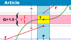
A function is continuous if it can be drawn in a single line without lifting the pencil. Hence, the green function $g$ in the following image is continuous and the red function $r$, which consists of two separate branches is discontinuous.

 

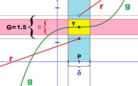
We have to admit that this definition by lifting a pencil is hardly something that can be called mathematics and fails in higher dimensions or for exotic functions which are defined differently on rational and irrational numbers. Nevertheless, it contains all we need to derive the mathematical definition. All we need is this picture with the green and the red function in mind.

 

The first thing that we have to accept is that continuity is a property that takes place somewhere, at a specific location, at a point $x=p.$ The term continuous function means it is everywhere continuous, at all locations of $x.$ Speaking of a continuous function disguises the local aspect of continuity which is crucial. Lifting the pencil takes place somewhere, not everywhere. This also shows that it is easier to describe the discontinuity of the red function $r$ than it is to describe the continuity of the green function $g$. The second thing is another distance $\delta >0$ besides $\varepsilon >0$ since we need to talk about the $x$-axis and the $y$-axis, i.e. about distances in the domain of the function, and distances in the codomain of the function if we want to get a hold on lifting the pencil. This leads us to our third observation. The gap $G=1.5$ takes place in the codomain. The projections of the functions onto the $x$-axis are unremarkable. However, the gap allows a (yellow) rectangle $Y$ with side lengths $\delta$ and $\varepsilon$ where we cannot find any points of the red function $r(x)$ although the function is defined in all points of the $\delta$-interval. This is our chance to define lifting the pencil, the gap $G$.

Definition A: A function is discontinuous at $p$ if there is a gap between function values that cannot be dropped below no matter how close to $p$ we look to take the values in the domain.

Definition B: A function $r : D\rightarrow C$ is discontinuous at $p\in D$ if there is a $G>0$ such that $|r(x)-r(p)|>G$ for all $|x-p|<\delta .$

Now all we have to do in order to define continuity is to take the logical negation of our definition.

Definition C: A function $g : D\rightarrow C$ is continuous at $p\in D$ if for every $\varepsilon >0$ there exists a $\delta =\delta(p,\varepsilon )>0$ such that
$$
|g(x)-g(p)|<\varepsilon \quad \forall\;x\; \text{with} \; |x-p|<\delta(p,\varepsilon).
$$
Note that the distance $\delta$ on the $x$-axis (in the domain) depends on the choice of the distance $\varepsilon$ on the $y$-axis (in the codomain) as well as on the choice of the location $p$. Continuous functions for which $\delta$ does not depend on the location are called uniformly continuous. An example of a continuous function that is not uniformly continuous is
$$
g(x)\, : \,(0,1] \rightarrow \mathbb{R}\, , \,g(x)=\dfrac{1}{x}
$$
because $\delta$ cannot be chosen uniformly for all locations.
The closer we want to have our function values, the closer we usually need to demand our domain values around $p$ to be. But it all starts with an arbitrarily small distance $\varepsilon >0$ again, and the request for the existence of a dependent number $\delta (p,\varepsilon)>0.$

 

The above considerations were forced by our general subject, the $\varepsilon -\delta$ world. However, the gap was crucial for our understanding of discontinuity and continuity. But drawing a line and lifting the pencil is also a limit process. We come closer to $x=p$ and all of a sudden we find a gap $G$ in the graph of the discontinuous red function, and none in the graph of the continuous green function. One disturbs our limit process, the other does not. This allows us

Definition D: A function $g : D\rightarrow C$ is continuous at $p\in D$ if
$$
\lim_{x \to p}g(x) =g(p).
$$
This notation is a bit tricky. It looks simple but it has implicit assumptions, namely that the limit from the left and the limit from the right a) both exist and b) coincide. Therefore it is better to write

Definition E:  A function $g : D\rightarrow C$ is continuous at $p\in D$ if
$$
\lim_{x \nearrow p}g(x) =\lim_{x \searrow p}g(x)=g(p).
$$
We haven’t defined what the limit of a function is, so let us explain this with sequences.

Definition F: A function $g : D\rightarrow C$ is continuous at $p\in D$ if for every sequence $(a_n)_{n\in \mathbb{N}}\subseteq D$ in the domain, that converges to $p,$ the function values converge to $g(p),$ i.e.
$$
\lim_{n \to \infty}a_n=p\quad \Longrightarrow \quad \lim_{n \to \infty}g(a_n)=g(p).
$$
The possible directions for our approach to the point $p$ are hidden here in the request that this has to hold for every sequence that converges to $p,$ no matter whether from left, form right, or from other directions in higher dimensions. It would be a valuable exercise to prove the equivalence of the definitions C and F, and why the red function is not continuous at $p$ in this sense before we come to the more theoretical part of this article.

Topology, and Continuity Revisited

A category is a collection of objects of a certain kind and the mappings between those objects. Topological spaces are an example of a category. A topological space is a set and a collection of subsets called a topology which contains the empty set, the entire space, i.e. the full subset and is closed under finite intersections and arbitrary unions. The sets in a topology are called open sets. The mappings in the category of topological spaces are precisely the (everywhere) continuous functions. A function is continuous if the pre-images of open sets are open, too.

 

This was probably the briefest summary of the mathematical background of a continuous function that is imaginable. Nothing reminds us of the $\varepsilon -\delta$ world, the distances, or even intervals on the coordinate axis we considered in the previous sections! But this isn’t an article about topology, so we will not hesitate to fill this very abstract concept of a topological space with specific content. Our topological space is the set of real numbers, and if we wanted to consider more abstract concepts, we would choose higher real dimensions or complex numbers, for short: a space that admits distances, so-called metric spaces. Our topology on the set $\mathbb{R}$ is
$$
\displaystyle{\mathcal{T}(\mathbb{R})=\left\{\emptyset\, , \,\mathbb{R}\, , \,\displaystyle{\bigcup_{\kappa\in K}} I_\kappa\right\}}
$$
where $I_\kappa= (a_\kappa,b_\kappa)=\{x\, : \,a_\kappa\leq x\leq b_\kappa\}$ are any open intervals and $K$ is an arbitrary index set. Even uncountably many indexes are allowed. A metric changes the situation instantly. If we have an open set, then every point of such a set is contained in an open interval that entirely lies inside that open set. Between $|a|<|x|$ is always room for another $|a|< |a’|<|x|$. And since we are allowed to build arbitrary unions of open sets, the opposite is also true. Metric spaces are nice examples of topological spaces. A positive, symmetric, and the triangle inequality obeying distance function allows us to describe open sets precisely. All we need is an open interval (open ball) around each point of them. Thus, definition C for the continuity of a function $g:D\rightarrow C$ where $D,C\subseteq \mathbb{R}$ at $p\in D$ can now be rewritten as

Definition G: A function $g : D\rightarrow C$ is continuous at $p\in D$ if for every $\varepsilon >0$ there exists a $\delta =\delta(p,\varepsilon )>0$ such that
\begin{align*}
I_\delta (p)&=\left(p-\delta /2,p+\delta /2\right) \subseteq g^{-1}(I_\varepsilon (g(p)))\\
&=g^{-1}\left(g(p)-\varepsilon /2,g(p)+\varepsilon /2\right)
\end{align*}
which means that $g^{-1}(I_\varepsilon (g(p)))$ is an open set.

 

A look at the picture above shows us that
$$
r^{-1}\left(r(p)-G/2 , r(p)+G/2\right) =r^{-1}\left(\left(r(q),r(p)\right]\right) = \left(q,p\right]:=J
$$
for some point $q\in D.$ This set is not open because $p$ is not contained in an open interval that entirely lies within this half-open interval $J.$ The red function $r$ is not continuous at $p.$

Topology and continuous functions belong together, and continuity is defined by open sets. We need the key of a metric that allows us to specify open sets of certain topological spaces – metric spaces – in order to enter the $\varepsilon -\delta$ world. We only considered the real absolute value function as our metric but everything remains true for arbitrary metrics, like e.g. the complex absolute value, or the Euclidean distance in higher dimensional real vector spaces, and of course for Hilbert spaces, too.

Limits – revisited

I owe you some explanations about the importance of limits, and why we can prove convergence without knowing the limit although it shows up in the definition of convergence. The latter is the so-called Cauchy criterion for sequences. A sequence of real or complex numbers converges to a limit if and only if
$$
\forall \,\varepsilon > 0 \quad\exists \, N(\varepsilon )\in \mathbb{N}\, : \,|a_{m}-a_{n}|<\varepsilon \quad\forall\,m,n>N(\varepsilon )\quad (***)
$$
Sequences with the property $(***)$ are called Cauchy sequences. A limit $L$ does not occur in the defining statement anymore. Instead, it is hidden in the requirement that we have real or complex numbers. It can indeed be used to define the topological completion of the real, and therewith the complex numbers. They are exactly the number set that we get if we add all such possible limits $L$ of Cauchy sequences to the rational numbers. The Cauchy-criterion is therefore either a useful tool if you already have real numbers, or a tautological statement if it defines the real numbers. It is clear that it does not work for rational numbers. E.g. we can construct a converging sequence $(a_n)_{n\in \mathbb{N}}\subseteq \mathbb{Q}$ of rational numbers with the Newton-Raphson algorithm, and thus a Cauchy sequence, such that
$$
\displaystyle{\lim_{n \to \infty}a_n=\sqrt{2}}
$$
has a limit that is not a rational number anymore.

Cauchy sequences are very important in real or complex analysis since they allow us to prove convergence even if we do not know the limit. However, it is not the primary reason why limits of sequences are important. Series are! A series is an expression
$$
\sum_{n=1}^\infty a_n
$$
where the summands $a_n$ can be anything from numbers of some kind, vectors, polynomials, functions in general, or operators; as long as we have a metric to define close. The question that comes naturally with them is whether a value $v$ can be attached to a series
$$
\sum_{n=1}^\infty a_n \stackrel{?}{=}v .
$$
But how could we find out whether and which value should be related? We cannot add infinitely often. Hence, we are forced to make it finite. We define the so-called partial sums
$$
S_N :=\sum_{n=1}^N a_n
$$
and continue to investigate the newly appeared sequence $(S_N)_{N\in \mathbb{N}}.$ If it has a limit $L$ then we set $v:=L.$
$$
\lim_{N \to \infty}S_N =L \quad \Longleftrightarrow \quad \sum_{n=1}^\infty a_n =L
$$
$$
\exists \,v=L\quad \forall \,\varepsilon > 0 \quad\exists \, N(\varepsilon )\in \mathbb{N}\, : \,\left|\sum_{k=1}^n a_k -v \right|<\varepsilon \quad\forall\,n>N(\varepsilon )
$$
Well, series deserves an article on their own, so we just mention Taylor series, Maclaurin series, Laurent series, or simply power series in general and give an example. Functions have long been identified by their related power series. Limits of sequences are important since the convergence of series is defined by the convergence of the partial sum sequence.

Example

The $\varepsilon -\delta$ world is primarily a proof technique to get a mathematical hold on distances and the closer and closer part of our intuition. However, we sometimes need actual numbers to determine what closer means numerically. Let us consider the exponential function
$$
x\;\longmapsto\; \sum_{n=0}^\infty \dfrac{x^n}{n!}=\sum_{n=0}^N \dfrac{x^n}{n!}+\underbrace{\sum_{n=N+1}^\infty \dfrac{x^n}{n!}}_{=:\,r_{N+1}(x)}
$$
and see what we need for
$$
\left|r_{N+1}(x)\right|< 2\dfrac{x^{N+1}}{(N+1)!}
$$
We estimate the remainder with a geometric series and for $|x|<1+\dfrac{N}{2}$
\begin{align*}
\left|r_{N+1}(x)\right|&\leq \sum_{n=N+1}^\infty \dfrac{|x|^n}{n!}\\
&=\dfrac{|x|^{N+1}}{(N+1)!}\cdot\left(1+\dfrac{|x|}{N+2}+\ldots +\dfrac{|x|^k}{(N+2)\cdots (N+k+1)}+\ldots\right)\\
&\leq \dfrac{|x|^{N+1}}{(N+1)!}\cdot\left(1+\left(\dfrac{|x|}{N+2}\right)^1+\ldots +\left(\dfrac{|x|}{N+2}\right)^k+\ldots\right)\\
&< \dfrac{|x|^{N+1}}{(N+1)!}\cdot \left(1+\dfrac{1}{2}+\dfrac{1}{4}+\ldots+\dfrac{1}{2^k}+\ldots\right)=2\dfrac{|x|^{N+1}}{(N+1)!}
\end{align*}
We therefore have for $|x|<\delta$ with $\delta =\delta(0,\varepsilon ):=\varepsilon /2$
$$
\left|e^x-1\right|=\left|\sum_{n=1}^\infty \dfrac{x^n}{n!} \right| = |r_1(x)| < 2|x| < \varepsilon
$$
which proves the continuity of the exponential function at $x=0$ and
$$
\lim_{x \to 0} e^x=1
$$
by definition D. The continuity elsewhere can now be derived with the functional equation of the exponential function. We use again definition D and assume an arbitrary sequence $(a_n)_{n\in \mathbb{N}}$ that converges to a point $p.$ Then $a_n-p$ is a sequence that converges to $0$ and we just saw that then
$$
\lim_{n \to \infty}e^{a_n-p}=1
$$
hence
\begin{align*}
\lim_{n \to \infty} e^{a_n}=\lim_{n \to \infty}e^p\cdot e^{a_n-p}=e^p \lim_{n \to \infty}e^{a_n-p}=e^p\cdot 1 = e^p.
\end{align*}
The estimation of the remainder can also be used to approximate
\begin{align*}
e&=\sum_{n=0}^{15}\dfrac{1}{n!} +r_{16}(1)<\dfrac{888656868019}{326918592000} \pm \dfrac{2}{16!}=2.718281828459 \pm 2\cdot 10^{-13}
\end{align*}