How to Solve Einstein’s Field Equations in Maxima

A few months ago, pervect pointed me to a post by Chris Hillman which is an introduction to the usage of Maxima for General Relativity. Maxima is a free (both as in beer and as in speech) symbolic algebra package, and it includes a library called censor that handles tensor components and looks to have been written with General Relativity in mind. In his post, Hillman uses it to derive the Schwarzschild solution in Painleve coordinates and the Kerr solution for a rotating black hole.

As I’m the type of person who loves a worked example to take apart and re-build, I was very excited to be given exactly that for a solution of Einstein’s Field Equations. I decided to have a play, partly to learn Maxima and ctensor, and partly to learn a bit more about General Relativity.

I thought it would be worth writing an Insight about what I did since I didn’t know about the original article and I think it’s worth linking to in something more recent. There’s no need to read the original article before this one, but if you find this one interesting it’s probably worth a look. I’ll also say at the outset that there are quite a few criticisms that one could make of my method here. I’ve commented on some at the end. But I thought it was worth leaving as is because the bull-headed approach worked, and more elegant approaches can be built on it.

Field of Frames

A little bit of theory is needed before diving into Maxima.

The manifolds in general relativity are always locally flat; that is you can always create a small flat Minkowski frame at any point. You can’t extend them very far because curvature becomes apparent, but you can create another flat frame nearby with similar basis vectors. Rinse and repeat, and you can cover some part of spacetime with a collection of small frames – a frame field. If you arranged the basis vectors smoothly and systematically then you can smoothly relate them to global coordinates.

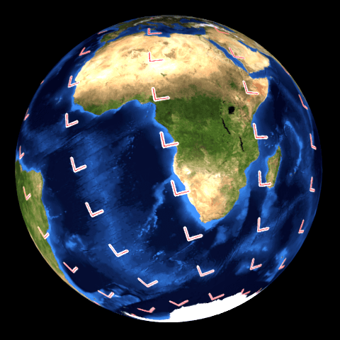
It’s traditional to illustrate this kind of thing with a sphere, and who am I to defy tradition. You can draw a nearly accurate flat map centered at any point on a sphere such as the Earth, and you can always choose to use the flat map centered at your current location (that’s how Google maps et al work). And you can (almost!) always write a mathematical relationship between global coordinates (e.g. latitude/longitude) and local coordinates (x and y on your map). The picture below is of a lot of little red set-squares dropped across the surface of the Earth in a systematic pattern (there should be infinitely many infinitesimally small frames, but that’s fiddly to draw). These are each the basis of a local flat map – a frame. Their collection is a frame field.

I’ve also drawn a Mercator projection map, which treats the latitude and longitude coordinates as orthonormal. The frames aren’t the same as the coordinates so are distorted on the map. Just to be awkward, I picked a system of laying out the set-squares that don’t quite match up with the coordinates so the distortion is severe enough in some places that the frames almost don’t seem to line up.

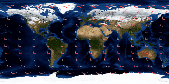
On the map, you can see that the set-squares vary in a complicated but systematic way. So I could express the length and direction of the rods at a point in terms of a smooth function of the latitude and longitude (the coordinates) of the point. Since frame fields are constructed from natural basis vectors, $\sigma^\mu$, for a locally flat coordinate system, the metric at that point is easy to express in terms of them:$$g=\sigma^0\otimes\sigma^0-\sum_{i=1}^3\sigma^i\otimes\sigma^i$$I find this a very useful concept, since it neatly relates the rather abstract concept of the metric to a local reference frame (something you can imagine someone in a hi-vis jacket and a theodolite working with) and through the frame field to the coordinates.

Build them…

The approach Hillman takes in his article is to pick an ansatz (a German word that boils down to “working model, details to be filled in later”) for the frame field expressed in some coordinate system. Then he sets up the Einstein field equations in terms of the ansatz and solves them to fill in the details. Hillman actually works with the co-frame field because that’s what ctensor uses, but that doesn’t make any difference to the strategy.

So what’s the ansatz for the interior of a body like a (non-rotating) planet or star? Let’s think about physics. The matter in the interior of the sphere is spherically symmetric and isn’t moving. That means it makes sense to work in something like Schwarzschild coordinates for this since this is a static, spherically symmetric coordinate system where an object with unchanging spatial coordinates is hovering at constant altitude. Since the coordinates reflect the physics, there should be (hopefully!) a fairly straightforward relationship between the coordinates, the frame field, and the physics.

Schwarzschild coordinates use the obvious angular coordinates on a sphere. The radial coordinate is the area of the sphere divided by $4\pi$ (this would just be the radius of the sphere in flat spacetime, but isn’t necessarily so in curved spacetime). The time coordinate is orthogonal to the three spatial ones. If we’re going to use a frame field it would make sense not to get cute (as I did with my red set-squares), and to align our frame field with the physics which happens to be reflected in our coordinate system. But what are the (coordinate) lengths of the rods making up our frames?

The angular directions scale as $r$ and $r\sin\theta$ – by definition, since we chose the coordinates to do this. The $r$ and $t$ directions we expect to behave in a slightly more complex way – we expect the radial scale to be a function of $r$, not a constant. Similarly, we expect the time coordinate to vary as a function of $r$ (gravitational time dilation). We don’t expect either to vary as a function of time, though, since this is a solution where nothing is moving, so today is the same as tomorrow. Thus we can write down our ansatz for the co-frame field:$$
t_\mu=\left(\begin{array}{c}g_t(r)\\0\\0\\0\end{array}\right);\
r_\mu=\left(\begin{array}{c}0\\g_r(r)\\0\\0\end{array}\right);\
\theta_\mu=\left(\begin{array}{c}0\\0\\r\\0\end{array}\right);\
\phi_\mu=\left(\begin{array}{c}0\\0\\0\\r\sin\theta\end{array}\right)$$where $g_r(r)$ and $g_t(r)$ are to be determined.

The only other thing we need is the stress-energy tensor. We have non-rotating uncharged matter; just about the only thing that’s interesting about it is that it has a pressure term. The stress-energy tensor for dust (see, for example, Carroll’s equation 1.107) under pressure is$$T^{\mu\nu}=(\rho c^2+p)U^\mu U^\nu+pg^{\mu\nu}$$Now our earlier clever choice of coordinates pays off. The matter isn’t moving in these coordinates so the spatial components of its four-velocity are zero – so $U^\mu=\left(\sqrt{g^{00}},0,0,0\right)$. That means that $T^{00}=\rho c^2g^{00}$ and $T^{ii}=pg^{ii}$, and all the off-diagonal elements are zero. The presence of the metric components seems annoying. But ctensor provides the Einstein tensor in the lower index or mixed index form – and lowering an index on the stress-energy tensor gets rid of the metric components. So we have$$\begin{eqnarray*}T^0{}_0&=&-\rho c^2\\T^i{}_i&=&p\\T^\mu{}_\nu&=&0 \forall \mu\neq\nu\end{eqnarray*}$$

…and they will solve

Now we have the coframe field ansatz we can express the metric in terms of it and calculate the Einstein tensor. Then we can solve the Einstein Field Equations.

Generating the Einstein tensor isn’t difficult, just boring. You need all the Christoffel symbols (most are zero but you need to check) and all the independent components of the Riemann tensor. This is where Maxima starts to show its worth. The ctensor package does all this for you, and you can even get it to spit out TeX so you can mostly copy-paste the results. The code is in the collapsible block below.

I’ve commented it fairly thoroughly so I won’t go through it line by line, just note that it uses cframe_flag to tell ctensor we’re starting with a co-frame field, stores the co-frame one-forms in the rows of fri, and then just grinds through the maths. The ctensor documentation (http://maxima.sourceforge.net/docs/manual/maxima_26.html#SEC139) has a nice map showing what relies on what. The metric is stored in lg and the mixed einstein tensor in ein. The metric turns out to be $$g_{\mu\nu}=\pmatrix{-g_t^2&0&0&0\cr 0&g_r^2&0&0\cr 0&0&r^2&0\cr 0&0&0&r^2\,\sin ^2 \theta\cr }$$and the Einstein tensor in mixed form is diagonal with elements:$$\begin{eqnarray*}G^t{}_t&=&-\frac{2g’_rr+g_r^3-g_r}{g_r^3r^2}\\G^r{}_r&=&\frac{2g’_tr+\left(1-g_r^2\right)g_t}{g_r^2g_tr^2}\\G^\theta{}_\theta&=&\frac{\left(g_rg^{\prime\prime}_t-g’_rg’_t\right)r+g_rg’_t-g’_rg_t}{g_r^3g_tr}\\G^\phi{}_\phi&=&\frac{\left(g_rg^{\prime\prime}_t-g’_rg’_t\right)r+g_rg’_t-g’_rg_t}{g_r^3g_tr}
\end{eqnarray*}$$where a prime denotes differentiation with respect to $r$.

The Einstein field equations are $$G^\mu{}_\nu=\frac{8\pi G}{c^4}T^\mu{}_\nu$$Since both the Einstein tensor and the stress-energy tensor are diagonal, we get four equations:$$\begin{eqnarray}
-\frac{2g’_rr+g_r^3-g_r}{g_r^3r^2}&=&-\frac{8\pi G\rho}{c^2}\\
\frac{2g’_tr+\left(1-g_r^2\right)g_t}{g_r^2g_tr^2}&=&\frac{8\pi Gp}{c^4}\\
\frac{\left(g_rg^{\prime\prime}_t-g’_rg’_t\right)r+g_rg’_t-g’_rg_t}{g_r^3g_tr}&=&\frac{8\pi Gp}{c^4}\\
\frac{\left(g_rg^{\prime\prime}_t-g’_rg’_t\right)r+g_rg’_t-g’_rg_t}{g_r^3g_tr}&=&\frac{8\pi Gp}{c^4}
\end{eqnarray}$$Clearly the last one is redundant as it duplicates the third – but that’s expected for a spherically symmetric situation, since it’s saying that the behaviour is the same in any direction in the surface of a sphere.

The equations look quite complex, but there is some hope because the first one depends only on $g_r$ and its derivatives. Maxima has tools to solve ODEs, and it does indeed spit out a solution – two, in fact because it solves for $g_r^2$. Here’s the code:

In the previous code block, I defined the matrix efe to contain the 4×4 Einstein field equations. A minor annoyance of Maxima is that its arrays are numbered from 1, not 0, so the first line here solves the tt field equation (an Ordinary Differential Equation, ODE) for $g_r$ in terms of $r$. Since this turns out to yield an expression for $r$ in terms of $g_r^2$, the next line rearranges % (Maxima code for “the result of the previous line”) for $g_r$. The third line takes the RHS of the second expression (the positive square root) for $g_r$ and substitutes 0 for %c, which is the constant of integration, and stores the result in grs. That expression was $$g_r(r)=\sqrt{3}c\sqrt{-\frac{r}{8\pi r^3\rho G-3c^2r-3kc^2}}$$where $k$ is the constant of integration that Maxima called %c. We immediately suspect it is zero because otherwise, the expression is singular at the origin. That isn’t necessarily a problem (it could be just a bad choice of coordinates), but it would seem a little surprising. You can go further and calculate the Kretschman scalar, which contains a term like $kg_t(r)^2/r^6$, which would only be finite for non-zero $k$ if the $tt$ component of the metric is at least $O(r^3)$, which seems unlikely. There’s a better reason still, which I will discuss later. So we conclude that $$g_r (r)=\sqrt{\frac{3c^2r}{3c^2r-8\pi r^3\rho G}}$$

Next we can solve for $g_t(r)$ by eliminating $p(r)$ from (2) and (3) and substituting in our solution for $g_r(r)$. This yields a second order ODE that Maxima can again solve. Here’s the code:

This uses ode2 again; the only complications are using ratsimp (simplify rational functions) and substituting in the solution for $g_r$ and its derivative. This time ode2 gives an explicit solution for $g_t (r)$, so there’s no need to rearrange with solve. The result is:$$g_t(r)=k_1\frac{\sqrt{8\pi r^2\rho G-3c^2}}{8\pi\rho G}+k_2$$where $k_1$ and $k_2$ are constants of integration (Maxima calls these %k1 and %k2).

To determine these constants we can note two things. Firstly, the pressure at some radius $r$ is entirely due to the weight of matter above it, so must go to zero at the surface. We can solve (2) for $p(r)$ using

The solution is:$$p(r)=-\frac{8\pi k_2c^2\rho^2G\sqrt{8\pi r^2\rho G-3c^2}+24\pi k_1c^2r^2\rho^2G-9k_1c^4\rho}{24\pi k_2\rho G\sqrt{8\pi r^2\rho G-3c^2}+24\pi k_1r^2\rho G-9k_1c^2}$$Secondly, we note that because we are using Schwarzschild-like coordinates, the components of the metric tensor at the surface must be the same as the Schwarzschild vacuum solution at the surface.

So, defining the surface to lie at $r=r_g$, we can solve $p(r_g)=0$, $g_t^2(r_g)=1-2GM/c^2r_g^2$, and $g_r^2(r_g)=(1-2GM/c^2r_g)^{-1}$ to get $k_1$, $k_2$, and to get a relationship between $\rho$ and $M$. The latter turns out to be $M=4\pi r_g^3\rho/3$, slightly surprisingly since this is the relationship in Euclidean space. Actually, the volume inside $r_g$ is larger than $4\pi r_g^3/3$, and if you took all the matter and spread it around in little chunks the total mass would be greater than M. But the pressure provides a negative contribution to the energy that cancels out the “extra” mass that fits in the “extra” space. The code to do all this is:

Again, I won’t go through this line by line. The only new thing is the use of the radcan function to do some simplification – this one cancels radicals.

I shan’t write out $k_1$ and $k_2$. Substituting them back in to $g_t(r)$ is the last step we needed to do. The metric is diagonal with components:$$\begin {eqnarray*}g_{tt}&=&-\left(\frac 12\sqrt{1-\frac{2GMr^2}{c^2r_g^3}}-\frac 32\sqrt{1-\frac{2GM}{c^2r_g}}\right)^2\\g_{rr}&=&\left(1-\frac{2GMr^2}{c^2r_g^3}\right)^{-1}\\g_{\theta\theta}&=&r^2\\g_{\phi\phi}&=&r^2\,\sin ^2 \theta\end{eqnarray*}$$

Is it right?

Well, according to Wikipedia, yes (note it uses the opposite sign convention and the compact form of the metric). So it must be right [citation needed]. Wikipedia does cite Schwarzschild’s original paper, but the form Schwarzschild used is sufficiently different (algebraically) to be difficult to compare, and my German isn’t up to following it. But other sources do agree with Wikipedia (e.g. http://insa.nic.in/writereaddata/UpLoadedFiles/IJPAM/20005a6c_9.pdf, and Schutz’ textbook).

We can also do a sanity check by calculating the proper acceleration of a hovering observer at different radii, plugging in numbers for the Earth, and comparing it to the Newtonian case. We don’t expect an exact match (not least because Schwarzschild’s $r$ and Newton’s aren’t quite the same things), but for a weak field like the Earth’s, this shouldn’t make much difference.

The choice of Schwarzschild-like coordinates pays off again because a hovering observer is not changing spatial coordinates, so has four-velocity $U^\mu=\left(c/\sqrt{-g_{00}},0,0,0\right)$. The four-acceleration is given by $A^\mu=U^\nu\nabla_\nu U^\mu$, and the proper acceleration is just $a=\sqrt{g_{ij}A^iA^j}$. To carry out this calculation in Maxima I wrote a function to do the covariant differentiation and the acceleration and ended up writing another to substitute in the numbers. This is a bit complex, but the plotting is as easy as you might expect. The expression for acceleration is ugly enough and long enough that I won’t bother putting it here. The code, the resulting graph, and the fractional difference from the Newtonian case are below.

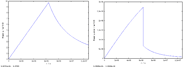
Note the scale ($3\times 10^{-8}ms^{-2}$) on the difference (right hand) graph. So this all looks good.

How did I do this?

I didn’t actually do very much. I tried this as an extension of an example by Chris Hillman of how to use Maxima for general relativity. I thought about a sensible choice of coordinates and a sensible frame field ansatz, and then just plugged that into the ctensor package in Maxima, pretty much cut-and-paste from Hillman, and it spat out the Einstein tensor. I worked out the stress-energy tensor and plugged that in. Then I just used the ode2 function to solve the various ODEs and used the various solutions and simplify functions to clean up. The only remotely clever programming I did was to write a couple of functions to take covariant derivatives and calculate the four-acceleration.

Naturally, it wasn’t all that plain sailing, and I went down a couple of blind alleys before I actually found the solution. And this is why I have fallen in love with computer algebra. Working by hand, the probability of me making a stupid algebraic slip would have been $\lim_{\epsilon\rightarrow 0}(1-\epsilon)$. So when something didn’t work, I would have had to spend a lot of time working out if it was the method that was actually wrong, or if I had failed to cancel something or made a transcription error.

This has revolutionized the way I approach a problem like this. I can be much more aggressive in trying to solve it, since it has drastically lowered the cost of trying something that turns out not to work. When an expression is growing rapidly more complex, I’m less worried that I’ve messed up the arithmetic and happier to accept that I’m going about it wrong.

This isn’t universally a good thing. The computer’s ability to handle complex algebra without silly mistakes means that I don’t have to be all that smart to get where I want to go. The solution I’ve described is somewhat bull-at-a-gate, and more elegant ways are possible – see the “A Better Way” section below.

And it has to be said that Maxima, while technically excellent, isn’t completely user-friendly. It’s pretty thoroughly documented, but Google seems to be the best way to actually find things in the docs. And Maxima itself is a text-only program. There are friendlier front-ends, and I used wxMaxima. But this has some tricksy behavior. For example, if you edit a command, you aren’t actually editing the command, you’re re-issuing it in its revised form. Which is fine, unless the command refers to the result of the previous one. Then you have to keep in mind that “the previous one” might be quite a lot further down the page than the command you’re editing…

I ended up developing a workflow where I developed in wxMaxima, and transferred “what worked” into a text editor and saved it as a .mac file. Then, every so often, I could restart Maxima (that’s a menu option in wxMaxima) and re-load the batch file to make sure Maxima was in the state I thought it was in. This is slightly clumsy, but it worked. If anyone has better ideas I’d be delighted to hear them.

A Better Way

I noted above that I hadn’t used the most elegant method to solve the problem. The first point (with thanks to PeterDonis for pointing this out) is that the tt component of the Einstein Field Equation admits a general solution of the form$$g_r(r)=\frac 1{\sqrt{1-m(r)/r}}$$where $m(r)$ is some as-yet-unidentified function of the radius that I just happen to have labeled as if it were something to do with mass. In fact, you can show that it’s the mass enclosed by the spherical surface at $r$, which immediately gives you a justification for setting the constant of integration $k$ to zero (no mass is enclosed in a sphere of radius zero) and for matching the metric components to the exterior Schwarzschild solution at the surface (you’re not matching two coordinate patches in this approach). In fact, I saw this approach myself in Michael Guidry’s notes on neutron stars and relativity, but didn’t spot the significance.

Also, the approach with frame fields was probably overkilled here. I could have gone straight to an ansatz for the metric, set cframe_flag to false, and saved me a bit of faffing.

The last thing was something I could have done better with Maxima. I noticed that there’s another package called itensor which does index manipulation, and can generate ctensor-friendly code. So I could, I think, have generated the code for calculating the acceleration four-vector this way. As I’m still very much learning Maxima, I’m sure there’s loads more about the code that will make experienced hands wince.

The end

I really enjoyed doing this, and I want to thank pervect again for pointing me to Chris Hillman’s article, Hillman himself for writing it, and PeterDonis for advice. I must say that when I signed up to Physics Forums six or seven years ago, I didn’t think I would be in a position to be finding solutions to Einstein’s equations in just a few years. Even if this is a solution that Schwarzschild already found (in a TRENCH! With PEN AND PAPER!), I’m really excited to be able to do this. And, in large part, I’ve done it with free (usually in both senses) resources – Carroll’s lecture notes, Ben Crowell’s GR text, listening and talking on here, Maxima, gnuplot. Even the Earth picture was done with a mix of Blender and python.

Sturgeon’s Law applies to the internet. But there’s a lot of good stuff in the other 10%.

References

Chris Hillman’s original Maxima/ctensor introduction: https://www.physicsforums.com/threads/brs-using-maxima-for-gtr-computations.378991/
Wikipedia’s page on the interior Schwarzschild metric: https://en.wikipedia.org/wiki/Interior_Schwarzschild_metric
Neutron stars and GR (lecture notes by Prof Michael Guidry, University of Tennessee Knoxville): http://eagle.phys.utk.edu/guidry/astro421/lectures/lecture490_ch10.pdf
Proper acceleration: https://www.math.ku.edu/~lerner/GR/Schwarzschild.pdf
Earth model: https://free3d.com/3d-model/planet-earth-99065.html