Particle in a Box: 1D & 2D Quantum Visualizations

Introduction

The particle in a box is a staple of entry-level quantum mechanics courses because it provides a clear contrast between classical and quantum dynamics. It is one of the few problems that can be solved exactly, without approximations. I suspect most readers solved only the 1-D particle-in-a-box in class and did not explore the larger picture, visualizing solutions, or higher-dimensional examples. Others reading this may work in a scientific field other than physics but are curious about the peculiarities of quantum mechanics.

In this Insight I briefly outline why the particle-in-a-box problem is important, what the solutions mean, and what the solutions look like in higher dimensions (2-D). Along the way you can pick up MATLAB code for making your own visualizations.

Why classical intuition fails

In the 1-D model the particle is free to move (potential energy V = 0) along a line of length L_x. No forces act on the particle inside the box; the walls are treated as impenetrable because the region outside the box has infinitely large potential (V = ∞).

Classical mechanics says that a particle in a 1 m box can have any speed and is equally likely to be found at any position along the line. That prediction changes dramatically when the box length is on the order of a nanometer (1×10^-9 m), where quantum mechanics applies. The quantum solution gives several nonintuitive results:

Key quantum results

1. The particle is more likely to be found in certain positions than others, depending on its energy.
2. There are nodes—positions where the probability density is always zero.
3. The particle’s energy is restricted to a discrete set of allowed energy levels (quantization).
4. The particle cannot have zero energy; it always has nonzero motion (zero-point energy).

The Schrödinger equation and separation of variables

We solve the problem using the time-dependent Schrödinger equation. I omit many mathematical steps; the references below fill in details.

i ħ ∂Ψ(x,t)/∂t = −(ħ² / 2m) ∂²Ψ(x,t)/∂x² + V(x) Ψ(x,t)

Here the variables are:

• Ψ — the wave function (encodes position, momentum, and energy information)
• V — potential energy
• x — position
• t — time
• ħ — reduced Planck’s constant
• m — particle mass
• i — imaginary unit

With a time-independent potential we use separation of variables, assuming Ψ(x,t) = ψ(x) φ(t). Substituting and separating gives a spatial eigenvalue equation and a time equation, both equal to the same constant E (the energy):

−(ħ² / 2m) d²ψ(x)/dx² + V(x) ψ(x) = E ψ(x)

i ħ dφ(t)/dt = E φ(t)

The spatial solutions are time-independent and are therefore called stationary states; each corresponds to a definite energy.

The 1-D wavefunction and boundary conditions

Solving the spatial equation in a region of zero potential yields a general solution:

ψ(x) = A sin(kx) + B cos(kx)

Impenetrable walls impose boundary conditions ψ(0) = ψ(L_x) = 0, which forces B = 0 and restricts the wavenumber to k = n π / L_x for integer n = 1, 2, 3, …. Thus

ψ_n(x) = A sin(n π x / L_x)

The corresponding energy levels are

E_n = ħ ω = (ħ² k²) / (2 m) = (n² π² ħ²) / (2 m L_x²)

Normalized stationary state

Choosing normalization constant A = sqrt(2 / L_x) gives the full time-dependent wavefunction for mode n:

Ψ_n(x,t) = sqrt(2 / L_x) sin(n π x / L_x) e^{−i ω t}

Simulating the 1-D solution

For visualization you can assign unit values to constants (for clarity) and plot the real part of Ψ(x,t) as it evolves in time. See the MATLAB code and animation below.

View the code for the 1-D time simulation

The 2-D particle in a box

In 2-D the particle is confined to a rectangle of width L_x and height L_y. The 2-D time-independent Schrödinger equation becomes

−(ħ² / 2m) (∂²ψ(x,y)/∂x² + ∂²ψ(x,y)/∂y²) + V(x,y) ψ(x,y) = E ψ(x,y)

Using separation of variables again, set ψ(x,y) = f(x) g(y). Each factor satisfies a 1-D-type equation, so the spatial eigenfunctions are products of sines:

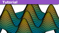
Ψ_nx,ny(x,y,t) = sqrt(4 / (L_x L_y)) sin(k_x x) sin(k_y y) e^{−i ω t}

Here k_x = n_x π / L_x, k_y = n_y π / L_y, and n_x, n_y = 1, 2, 3, …. The probability density has more nodes in 2-D, forming a grid of nodal lines depending on the two quantum numbers.

Simulating the 2-D solution

You can extend the 1-D MATLAB code to 2-D by evaluating the product sin(k_x x) sin(k_y y) on a grid and animating the real part in time.

View the code for the 2-D time-simulation for (n_x, n_y) = (4,4)

For multiple mode combinations see the full simulation code and the combined animation below.

View code for the full 2-D time-simulation

Feedback

Please leave comments or send me a message with any feedback so I can improve future posts.

Learn More

1. 2-D wells — University of Virginia
2. Particle in a box — Wikipedia
3. HyperPhysics: Particle in a box
4. Short video demonstration
5. Supplementary notes: Particle in a Box (2-D)