Learn the Basics of Hilbert Spaces and Their Relatives

 

Basics

Language first: There is no such thing as the Hilbert space.

Hilbert spaces can look rather different, and which one is used in certain cases is by no means self-evident. To refer to Hilbert spaces by a definite article is like saying the moon when talking about Jupiter, or the car on an automotive fair. The is either related to a unique subject or a context-sensitive certain one if there is no doubt about which one. The least should be a notation like e.g. Hilbert space of wave functions, of square-integrable functions, of Hilbert-Schmidt operators, or any other example, although even these neglect crucial information to some extend.

Hilbert spaces on the other hand are inevitably interwoven with quantum physics, be it the classical or the relativistic formalism. Whereas Gauß law and Maxwell’s equations could be viewed as expressions in the language of differential geometry, Schrödinger’s equations brought us wave functions and Hilbert spaces. I like to point out the interesting observation of the timely parallels between mathematical and physical developments, which led to all of them. It is a fascinating give and take which did not start with and continues up today in realms as gauge theories, Lie theory, representation theory, string theories or homological algebra, and the topological questions in cosmology.

Occasionally I get the impression that the concept of Hilbert spaces confuses students a bit. I’m not sure whether this is due to quantum physics, the missing restriction of finite dimensionality, the nature of their elements, or a mixture of all of them. So let’s see what Hilbert spaces actually are.

1. Vector Spaces.

Hilbert spaces $\mathcal{H}$ are at first real or complex vector spaces, $\mathbb{R}^n$ or $\mathbb{C}^2$ are Hilbert spaces. So all the theorems and definitions of linear algebra apply to the finite-dimensional ones and many to the infinite-dimensional ones, and we start at known ground. Let’s note the scalar field by $\mathbb{F} \in \{\mathbb{R},\mathbb{C}\}$ and for later use the complex conjugation as $z \mapsto \overline{z}$ and complex conjugate, transposed matrices as $A \mapsto \overline{A}^\tau= A^\dagger$.

Thus our first requirement for a Hilbert space is simply
$$
\forall\, {u,v \in \mathcal{H}}\, : \, u + v \in \mathcal{H} \\
\forall\, {\alpha \in \mathbb{F}, u \in \mathcal{H}} \, : \, \alpha \cdot u \in \mathcal{H}
$$
Vectors and scalars are still vectors and scalars, Hilbert space or not. The fact, that wave functions are noted as $\psi$ don’t change the fact, that as an element of some Hilbert space, they are considered to be vectors: straight directions pointing somewhere. We simply make use of the fact, that functions form a vector space; actually an algebra. They can be added, multiplied, stretched, and compressed. The natural mappings between them are therefore linear functions, whether we call them linear transformation or linear operator. The definition of a Hilbert space doesn’t say anything about dimensions. But neither does the definition of an ordinary vector space. Hilbert spaces can be finite as well as infinite-dimensional. Even functions as elements don’t guarantee infinite dimension. E.g. all polynomials of a degree less than three define a $3-$dimensional vector space which is basically $\mathbb{F}^3$ and thus a Hilbert space. However, in the infinite-dimensional case, we cannot simply write linear mappings as matrices, which is why another notation is normally used for linear operators (cp. § 2). For any subset $\mathcal{I} \subseteq \mathcal{H}$ linear combinations are
$$
\psi = \sum_{\psi \in \mathcal{I}} c_\psi \psi = \sum_{i=1}^n c_i\psi_i \quad (c_\psi \stackrel{a.a.}{=} 0)
$$
with almost all $c_\psi =0$, which means all but finitely many. This has to be distinguished from series of functions, which is something else and may have countably many summands:
$$
\psi(x) = \sum_{\psi \in \mathcal{I}} c_\psi \psi(x) = \sum_{i=1}^\infty c_i\psi_i(x)
$$
The former is simply another vector, the latter forces us to think about convergence and whether this sum makes even sense. Of course, we can also build limits of functions, still elements, and thus vectors:
$$
\psi = \lim_{n \to \infty} \psi_n
$$
If the index set $\mathcal{I}$ contains uncountably many elements, sums and limits in their usual sense don’t make sense any longer. In this case, we entered the topological part of Hilbert spaces as topological vector spaces and measure theory.

2. Inner Product Spaces.

Hilbert spaces have an inner product (dot product, scalar product) which must not be confused with scalar multiplication.
$$
\langle \; , \; \rangle \, : \, \mathcal{H} \times \mathcal{H} \longrightarrow \mathbb{F}
$$
The result of this product of two vectors is a scalar, a real or complex number, which makes the difference to the product of an algebra where the result is again a vector. For short: An inner product is a

positive,
$$
\langle \psi,\psi \rangle \geq 0
$$
definite,
$$
\langle \psi,\psi \rangle = 0 \Longleftrightarrow \psi = 0
$$
Hermitian,
$$
\langle\psi ,\chi \rangle = \overline{\langle \chi , \psi \rangle}
$$
sesquilinear form
$$
\langle \varphi , \alpha \psi + \beta \chi \rangle = \alpha \langle \varphi , \psi \rangle + \beta \langle \varphi , \chi \rangle
$$
i.e. linear in one argument. The behavior in the other argument follows from the Hermitian condition. Which one (first or second) is taken to be the linear argument and which one has to be complex conjugated depends on the author. The condition of Hermitian turns into a symmetrical requirement for real Hilbert spaces and we get an ordinary real inner product. The positive definiteness directly allows us to define a norm, a length of vectors, and a distance
$$
\parallel \psi \parallel = \sqrt{\langle \psi,\psi \rangle}
\\
d(\psi,\chi)=\parallel \psi-\chi \parallel
$$
This metric is called induced by the norm and an immediate consequence is, that Hilbert spaces are normed, topological vector spaces The topology allows us to speak about open and closed sets and continuous functions. In case the inner product is real-valued, e.g. if $\mathcal{H}$ is a real vector space, we even have an angle defined by
$$
\cos \sphericalangle (\psi,\chi) = \dfrac{\langle \psi,\chi \rangle}{\parallel \psi \parallel \cdot \parallel\chi \parallel}
$$
However, in any case, real or complex, we can define orthogonality simply by
$$\psi \perp \chi \Longleftrightarrow \langle \psi,\chi \rangle = 0\,$$
which allows us to speak of orthogonal complements of subspaces or an orthonormal basis in any Hilbert space. Hilbert spaces are also locally convex, which is an important property in functional analysis. Roughly speaking local convexity means, that open sets around a point contain an open ball, which rules out pathological topologies and accordingly strange functions. Linearity and norm guarantee this for Hilbert spaces.

Projection Theorem. Let $\mathcal{A}$ be a closed subspace of $\mathcal{H}$ and the orthogonal complement of $\mathcal{A}$ is $A^\perp = \{\psi \in \mathcal{H}\,\vert \,\psi \perp \chi \text{ for all } \chi \in \mathcal{A}\}$. Then $(\mathcal{A}^\perp)^\perp = \mathcal{A}$ and all elements $\psi \in \mathcal{H}$ can be uniquely written as $\psi = \chi + \varphi \in \mathcal{A}^\perp + \mathcal{A}$ and $\varphi$ is called the orthogonal projection of $\psi$ on $\mathcal{A}$. $\, \square$

As with every vector space $\mathcal{H}$, we also have a dual vector space $\mathcal{H}^*$. It consists of all linear functions into the underlying scalar field, i.e. $\mathbb{R}$ or $\mathbb{C}$. They are called functionals. On the other hand the inner product defines functionals in a natural way:
$$
v \longleftrightarrow v^*\, := (\,w \longmapsto \langle v,w \rangle \,)
$$
The following theorem connects the two.

Fréchet-Riesz Representation Theorem.
Let $\mathcal{H}$ be a Hilbert space. Then there is a unique element $\psi \in \mathcal{H}$ for every continuous functional $\psi^* \in \mathcal{H}^*$ such that
\begin{align}
\psi^* (\chi) &= \langle \psi, \chi \rangle ~~\forall \,\chi \in H \\
|| \psi^* || &= ||\psi||
\end{align}
On the other hand $\psi^*\, : \, \chi \longmapsto \langle \psi, \chi \rangle$ for any given $\psi \in \mathcal{H}$ defines a continuous functional with operator norm $||\psi^*||=||\psi||\,$. $\, \square$

The representation theorem is one way to justify the $\langle bra|ket \rangle$ formalism, the Dirac notation – I didn’t omit the ${}^*$ here for the sake of clarity
\begin{align}
\psi^* (\chi) = \langle \psi, \chi \rangle = \langle \psi^*| \chi \rangle = \langle \psi^*|( |\chi \rangle)=\overline{\langle \chi | \psi \rangle} \end{align}
The Dirac notation also allows to define the outer product, the rank $(1,1)$ tensor
\begin{align}
|\chi\rangle \langle \psi^*| := \chi \otimes \psi^* = \chi \cdot (\psi^*)^\tau \in \mathcal{H} \otimes \mathcal{H}^*
\end{align}
which is a matrix of rank $1$ that can be obtained by ordinary matrix multiplication, if the vectors $\chi, \psi^*$ are written as column vectors. It represents the linear map
\begin{align}
\varphi \longmapsto |\chi\rangle \langle \psi^*|(\varphi) = \chi \otimes \psi^*.\, \varphi = \psi^*(\varphi) \cdot \chi
\end{align}
We have already used some terms, which are not directly related to vector spaces as continuity or operator norm. However, we do not only have a vector space, the norm also allows a metric and therefore a topology on $\mathcal{H}$. It gives us the tool to define open sets, which allows us to speak about continuous functions and also supplies a measure for convergence properties.

3. Geometry and Topology.

We’ve already almost done the geometric part: we have, points, directions, distances and angles, which allows us to do geometry and prove theorems as:

Orthonormal Basis. Let $\mathcal{H}$ be a Hilbert space. Then to every finite or countable set $\{\psi_n\}\subseteq \mathcal{H}$ there is a finite or countable orthonormal system $M=\{\varepsilon_n\}$ with $\operatorname{span}F=\operatorname{span}M$ and the maximal orthonormal systems, which define a Hilbert space dimension, are exactly the orthogonal bases. If $F$ is linear independent we can achieve $\operatorname{span}\{\psi_1,\ldots\, , \,\psi_n\}=\operatorname{span}\{\varepsilon_1, \ldots ,\varepsilon_n\}$ for all $n$ and $M$ is even unique, if we require $a_n> 0$ in the expressions $\varepsilon_n = \sum_{k=1}^n a_k\psi_k\,\, \square$

Jordan and v. Neumann. Parallelogram law. A norm $||\,.\,||$ on a vector space $\mathcal{H}$ can be generated by a inner product $\langle \,.\, \rangle$, if and only if the parallelogram identity holds:
\begin{align}
||\psi + \chi||^2+||\psi-\chi||^2=2\cdot (||\psi||^2+||\chi||^2)
\end{align}
The statement exceeds to seminorms and semi-inner products.$\, \square$

That’s our keyword. Until now, i.e. without the topological requirement of completeness, which I’ll explain after this little foray, we have defined a so-called Pre-Hilbert space, a vector space with an inner product. Now I want to explain what we will get if we reduce our norm to only a seminorm.

Definition. Seminorm. A seminorm is a real valued function $\sigma \, : \,\mathcal{H} \longrightarrow \mathbb{R}$ on a vector space $\mathcal{H}$, such that

• $\sigma (\psi) \geq 0$
• $\sigma(\lambda \psi) = |\lambda|\sigma(\psi)=\left(\sqrt{\lambda\cdot \overline{\lambda}}^{}\right) \sigma(\psi)$
• $\sigma(\psi+\chi) \leq \sigma(\psi)+\sigma(\chi)$

Each norm is a seminorm which is positive definite, so Hilbert spaces have one. With them we can define another geometric property of Hilbert spaces, namely that they are locally convex topological vector spaces. Topological simply means, that we know what the open subsets are in our space. However, I want to give a more geometric definition, which in my opinion is more intuitive and refer to the literature for the definition via seminorms.

Definition. Locally convex space. A topological $\mathbb{F}-$vector space $\mathcal{H}$ is locally convex, if every neighborhood of its origin $0$ contains an open set $T \subseteq \mathcal{H}$ which is

• convex, i.e. $T$ contains all line segments between any two points of it  $\\ \psi,\chi \in T \Longrightarrow \lambda \psi+(1-\lambda)\chi \in T \,\,\,\, \forall\, \lambda \in [0,1]\subseteq \mathbb{R}$
• absorbent, i.e. $\mathcal{H}$ can be covered by copies of $T$, or for all vectors there is a boundary such that all shorter vectors are elements of $T$ $\\ \forall \, \psi\in \mathcal{H} \,\exists \, \mu_\psi \in \mathbb{R}^+ \, : \, \forall \,|\lambda| < \mu_\psi \, : \,\lambda \psi \in T$
• balanced, i.e. $T$ contains all points of a disc (interval) centered at the origin and a given point of $T$ on its boundary  $\\ \forall \, \psi\in T \,\forall \, |\lambda|\leq 1\, , \,\lambda \in \mathbb{F}\, : \,\lambda \psi \in T$

The last ingredient to Hilbert spaces is completeness, which is a purely topological attribute and distinguishes Pre-Hilbert spaces from Hilbert spaces. It simply means that all Cauchy sequences converge and their limits are already part of the space, not outside. A Cauchy sequence is a sequence $(\psi_n)_{n \in \mathbb{N}} \subseteq \mathcal{H}$ whose elements get closer and closer: \begin{equation} \forall \,\varepsilon > 0 \, \exists \, N_\varepsilon\, : \,||\psi_n – \psi_m|| < \varepsilon \quad \forall \, n,m \geq N_\varepsilon
\end{equation}
It is the same as with rationals (incomplete) and reals (complete). We can have a sequence of rational numbers, which is a Cauchy sequence, e.g.
\begin{equation}
p_n := \dfrac{1}{1^2}+\dfrac{1}{2^2}+\dfrac{1}{3^2}+\ldots +\dfrac{1}{n^2}\quad (n \in \mathbb{N})
\end{equation}
which converges, but only in the reals, as its limit is
\begin{equation}
\lim_{n \to \infty}p_n = \zeta(2) = \dfrac{\pi^2}{6} \quad (Leonhard\, Euler, 1748)
\end{equation}
and therefore not rational. Here we have Pre-Hilbert spaces (possibly incomplete) and Hilbert spaces (complete). Since Pre-Hilbert spaces are a class of spaces, whereas the rational numbers are a specific field, Pre-Hilbert spaces merely do not need to be incomplete, they may as well be complete, in which case we call them Hilbert spaces. I follow the convention, that Pre-Hilbert spaces contain Hilbert spaces, and not that they are complementary. To have all limits actually available, if the elements of a sequence are closing down, is an important and convenient property. However, we have similar to the situation $\mathbb{Q}\subseteq \mathbb{R}$ the following theorem.

Completion Theorem. For every Pre-Hilbert space $\mathcal{H}$ there is a completion $\hat{\mathcal{H}},$ i.e. a Hilbert space which contains $\mathcal{H}$ and two completions of $\mathcal{H}$ are isomorphic.$\, \square$

Isomorphisms in this context are also isometries, that is a linear operator
\begin{align}
&T\, : \,(\mathcal{H}_1,||.||_1) \longrightarrow (\mathcal{H}_2,||.||_2)\\
&\text{T is defined on the entire space }\mathcal{H}_1\\
&||T\psi||_2 = ||\psi||_1
\end{align}
that is also a bijection with $\operatorname{im}T = \mathcal{H}_2$

Somehow related to Hilbert spaces are Banach spaces, especially are Hilbert spaces also Banach spaces. The distinction is, that we do not require an inner product for a Banach space, but merely a norm. Completeness holds for both of them.

Theorem. Two normed and isomorphic spaces are Banach spaces (Hilbert spaces) if and only if one of them is.$\, \square$

The fact that we have topological spaces involves many properties for closed subsets, dense subsets, and other topological features, and the fact the dimensions aren’t restricted to a finite number requires some attention on which theorems from linear algebra still hold, resp. in which form. The combination of linearity and topology is basically the origin of functional analysis.

4. An Overview.

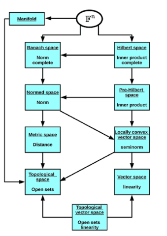
Arrows are inclusions: “is a”

5. Examples.

First of all, we have to find vector spaces. We need additions and stretches. Besides the usual vector spaces $\mathbb{F}^n$, there are also sequences and functions which satisfy these conditions. We have a variety of norms available, from absolute values, over Euclidean norms to maximum norms. All these summarize the basic examples for (Pre-)Hilbert and Banach spaces.

5.1. $\mathbb{F}^n$

\begin{equation}
\langle \psi,\chi \rangle = \sum_{j,k}^n a_{jk}\overline{\psi}_j \chi_k
\end{equation} gives us a sesqiliniear form on $\mathbb{F}^n$ which is Hermitian if and only if the matrix $(a_{jk})$ is. The most important case here is $(a_{jk})=I$. In this case we get the ordinary Euclidean angles and lengths.

5.2. $C_\mathbb{F}^0[0,1]$

This is the space of continuous $\mathbb{F}-$valued functions on $[0,1]$. If $\rho\, : \,[0,1] \longrightarrow \mathbb{F}$ is a certain continuous function, then we have with
\begin{equation}
\langle \psi,\chi \rangle = \int_0^1 \overline{\psi}(x) \chi(x) \rho(x) \,dx
\end{equation} a sesqiliniear form on $C_\mathbb{F}^0[0,1]$ which is Hermitian if and only if $\rho$ is real valued.

5.3. $C_\mathbb{C}^0[0,1]$

Let $\kappa\, : \,[0,1]\times [0,1]\longrightarrow \mathbb{C}$ be continuous. Then
\begin{equation}
\langle \psi,\chi \rangle = \int_0^1 \int_0^1 \kappa(x,y)\overline{\psi}(x) \chi(y) \, dy \,dx
\end{equation} a sesqiliniear form on $C_\mathbb{C}^0[0,1]$ which is Hermitian if and only if the kernel $\kappa$ is, i.e. $\kappa (x,y)=\overline{\kappa(y,x)}$.

The last two examples show, that there is more than one way to define an inner product. The same is true for norms. I will define the usual ones and how seminorms naturally occur.

5.4. Norms and Seminorms on $\mathbb{F}^n$. $||.||_p$

\begin{align}
||\psi ||_1 &= \sum_{j=1}^{n} |\psi_j|\\
||\psi ||_2 &= \sqrt{ \sum_{j=1}^{n}|\psi_j|^2}\\
||\psi ||_p &= \sqrt[p]{ \sum_{j=1}^{n} |\psi_j|^p}\\
||\psi ||_\infty &= \operatorname{max}\{\,|\psi_j|\,: \,1 \leq j \leq n\,\}\\
\sigma_{1,c}(\psi) &= \sum_{j=1}^{n} c_j|\psi_j| \quad (c_j \in \mathbb{R}_0^+)\\
\sigma_{\infty,c}(\psi) &= \operatorname{max}\{\,c_j|\psi_j|\,: \,1 \leq j \leq n\,\} \quad (c_j \in \mathbb{R}_0^+)
\end{align}
The last two define seminorms, which are norms if all weights $c_j$ are positive.

5.5. Norms and Seminorms on $C_\mathbb{F}^0[0,1]$. $||.||_p$

The same as in the previous example with integrals instead of sums, and a nonnegative, continuous function $\rho\, : \, [0,1] \longrightarrow \mathbb{R}$ instead of the weight vector $c$.

5.6. Pre-Hilbert and not Hilbert. $C_2^0[0,1]$

We consider the vector space of continuous, real functions on $[0,1]$ again with the inner product as defined in 5.2. (14) with the Euclidean norm, the 2-norm ($p=2$) indicated by the lower index. The upper index stands for the degree of differentiability, with $0$ for continuous, $1$ for continuous differentiable once, and so on until $\infty$ for smooth functions, i.e. infinitely often differentiable functions. The weight function for the Euclidean norm is $\rho \equiv 1\,$. Now we define the following sequence of continuous functions:
\begin{align}
\psi_1 (x) &\equiv 1 \\
\psi_n(x) &=
\begin{cases}
1, & 0 \leq x \leq \frac{1}{2} \\
1-\left(x-\dfrac{1}{2}\right)\cdot n, & \frac{1}{2} < x < \frac{1}{2}+\frac{1}{n} \\ 0, & \frac{1}{2}+\frac{1}{n} \leq x \leq 1 \end{cases} \quad (n>1)
\end{align}
This sequence is a Cauchy sequence as $||\psi_n – \psi_m|| < n^{-1}$ and its limit is
\begin{align}
\psi(x) &=
\begin{cases}
1, & 0 \leq x \leq \dfrac{1}{2} \\
0, & \dfrac{1}{2} < x \leq 1
\end{cases}
\end{align}
which is obviously not continuous anymore.

5.7. Banach and not Hilbert. $C_\infty^0[0,1]$

The vector space of continuous, real functions on $[0,1]$ with the maximum norm ($p=\infty$) is a complete, topological vector space, but the maximum norm isn’t induced by an inner product. $$||\psi||_\infty = \operatorname{max}\{\,|\psi(x)|\,: \,0 \leq x \leq 1\,\}$$

5.8. Banach and Hilbert. $\mathbb{R}^n\; , \;\mathbb{C}^n$

The finite-dimensional real or complex vector spaces are Banach spaces with the unweighted norms defined above (cp. 5.4.) as well as Hilbert spaces with the inner product defined above (cp. 5.1.). Unweighted means the matrix $(a_{jk})= I$ and the weights $c_j=1\,.$

 

5.9. $\mathit{l}_p$ spaces.

I have already mentioned that the sequences build a vector space, too. We now consider the complex vector space of complex, bounded sequences, i.e.
$$
\sum_{j=1}^{\infty} \psi_j^p < \infty
$$
equipped with the $p-$norm as in (5.4.(18)), except that the sum is a series and it is summed over all $n \in \mathbb{N}\,.$ These spaces are Banach spaces. In fact they are even Banach algebras as also an ordinary multiplication can be defined. For the special case of $p=2$ we get the $\mathit{l}_2$ space with
\begin{equation}
\langle\psi, \chi\rangle = \sum_{n\in \mathbb{N}} \overline{\psi_n} \chi_n \text{ and } ||\psi||_2^2 = \sum_{n\in \mathbb{N}} |\psi_n|^2
\end{equation}
which is a Hilbert space. As a side note, $\mathit{l}_2$ is up to isometric isomorphisms the only infinite dimensional separable Hilbert space, i.e. it contains a countable, dense subset.

For my next example of Lebesgue spaces $L_p$ I will assume $p=2$. The other ones are basically analog, but Lebesgue spaces require a bit of measure theory and I don’t want to go too deep into it here. However, in the case $p=\infty$, it requires a bit of an exception handling. All $L_p$ spaces are Banach spaces, and $L_2$ is also a Hilbert space.

 

5.10. Lebesgue space. $L_2(M)$

Let $M \subseteq \mathbb{R}^n$ be a Lebesgue measurable subset. Then we consider the function space $\mathcal{L}_2(M)$ of all measurable, complex valued functions on $M$ which are bounded, i.e. $\int_M |\psi(x)|^2\,dx < \infty\,.$ This is a vector space and for $\psi, \chi \in \mathcal{L}_2(M)$
\begin{equation}
\sigma (\psi,\chi) = \int_M \overline{\psi(x)}\chi(x)\,dx
\end{equation}
defines a semi-inner product. The reason why it’s no proper inner product are null sets. If we had a nonempty null set $N$, then the characteristic function $1_N$ on $N$ would satisfy $||1_N||=0$ although $1_N \neq 0_N$ and definiteness would be broken. In order to repair this, we define the subspace $\mathcal{N}_2(M) \subseteq \mathcal{L}_2(M)$ of all complex valued, bounded functions, which are zero almost everywhere. Then $\mathcal{N}_2(M) = \{\,\psi \in \mathcal{L}_2(M)\, : \, \sigma(\psi, \psi)=0\,\}\,.$ Then the equivalences classes
\begin{equation}
L_2(M) := \mathcal{L}_2(M) / \mathcal{N}_2(M)
\end{equation}
\begin{equation}
\langle [\psi],[\chi] \rangle := \sigma (\psi,\chi) = \int_M \overline{\psi(x)}\chi(x)\,dx
\end{equation}
define the Hilbert space $({L}_2(M),\langle .,. \rangle)$ of square integrable functions.

5.11. Function spaces. $C^n(M)$

$C^n(M)$ is the space of all $n-$fold continuous differentiable functions with $n \in \mathbb {N} \cup \{0,\infty \}$. If $M$ is compact, then we get a Banach space with the norm
\begin{equation}
||\psi || = \sup_{k \leq n}\, \sup_{x \in M} |\psi^{(k)}(x)|
\end{equation}

 

Sources.