Learn Renormalization in Mathematical Quantum Field Theory

February 8, 2018/9 Comments/in Physics Articles/by Urs Schreiber

Estimated Read Time: 64 minute(s)

Common Topics: def, prop, matrix, margin, auto

This is one chapter in a series on Mathematical Quantum Field Theory

The previous chapter is: 15. Interacting quantum fields.

16. Renormalization

In this chapter we discuss the following topics:

Epstein-Glaser normalization
Stückelberg-Petermann re-normalization
UV-Regularization via Counterterms
Wilson-Polchinski effective QFT flow
Renormalization group flow
Gell-Mann & Low RG Flow

In the previous chapter we have seen that the construction of interacting perturbative quantum field theories is given by perturbative S-matrix schemes (def. 15.3), equivalently by time-ordered products (def. 15.31) or equivalently by Feynman amplitudes (prop. 15.51). These are uniquely fixed away from coinciding interaction points (prop. 15.42) by the given local interaction (prop. 15.42), but involve further choices of interactions whenever interaction vertices coincide (prop. 16.1). This choice is called the choice of (“re”-)normalization (def. 15.46) in perturbative QFT.

In this rigorous discussion, no “infinite divergent quantities” (as in the original informal discussion due to Schwinger-Tomonaga-Feynman-Dyson) that need to be “re-normalized” to finite well-defined quantities are ever considered, instead, finite well-defined quantities are considered right away, and the available space of choices is determined. Therefore making such choices is rather a normalization of the time-ordered products/Feynman amplitudes (as prominently highlighted in Scharf 95, see the title, introduction, and section 4.3). Actual re-normalization is the change of such normalizations.

The construction of perturbative QFTs may be explicitly described by an inductive extension of distributions of time-ordered products/Feynman amplitudes to coinciding interaction points. This is called

Epstein-Glaser renormalization.

This inductive construction has the advantage that it gives accurate control over the space of available choices of (“re”-)normalizations (theorem 16.14 below) but it leaves the nature of the “new interactions” that are to be chosen at coinciding interaction points somewhat implicit.

Alternatively, one may re-define the interactions explicitly (by adding “counterterms”, remark 16.24 below), depending on a chosen UV cutoff-scale (def. 16.20 below), and construct the limit as the “cutoff is removed” (prop. 16.23 below). This is called (“re”-)normalization by

UV-Regularization via Counterterms.

This still leaves open the question of how to choose the counterterms. For that, it serves to understand the relative effective action induced by the choice of UV cutoff at any given cutoff scale (def. 16.26 below). This is the perspective of effective quantum field theory (remark 16.27 below).

The infinitesimal change of these relative effective actions follows a universal differential equation, Polchinski’s flow equation (prop. 16.30 below). This makes the problem of (“re”-)normalization be that of solving this differential equation subject to chosen initial data. This is the perspective on (“re”-)normalization called

Wilson-Polchinski effective QFT flow.

The main theorem of perturbative renormalization (theorem 16.19 below) states that different S-matrix schemes are precisely related by vertex redefinitions. This yields the

Stückelberg-Petermann renormalization group.

If a sub-collection of renormalization schemes is parameterized by some group ##RG##, then the main theorem implies vertex redefinitions depending on pairs of elements of ##RG## (prop. 16.31 below). This is known as

Renormalization group flow

Specifically scaling transformations on Minkowski spacetime yield such a collection of renormalization schemes (prop. 16.36 below); the corresponding renormalization group flow is known as

Gell-Mann & Low RG flow.

The infinitesimal behaviour of this flow is known as the beta function, describing the running of the coupling constants with scale (def. 16.32 below).

Epstein-Glaser normalization

The construction of perturbative quantum field theories around a given gauge fixed relativistic free field vacuum is equivalent, by prop. 15.25, the construction of S-matrices ##\mathcal{S}(g S_{int} + j A)## in the sense of causal perturbation theory (def. 15.3) for the given local interaction ##g S_{int} + j A##. By prop. 16.1 the construction of these S-matrices is inductively in ##k \in \mathbb{N}## a choice of extension of distributions (remark 16.2 and def. 16.10 below) of the corresponding ##k##-ary time-ordered products of the interaction to the locus of coinciding interaction points. An inductive construction of the S-matrix this way is called Epstein-Glaser-(“re”-)normalization (def. 15.46).

By paying attention to the scaling degree (def. 16.4 below) one may precisely characterize the space of choices in the extension of distributions (prop. 16.12 below): For a given local interaction ##g S_{int} + j A## it is inductively in ##k \in \mathbb{N}## a finite-dimensional affine space. This conclusion is in theorem 16.14 below.

Proposition 16.1. ((“re”-)normalization is an inductive extension of time-ordered products to diagonal)

Let ##(E_{\text{BV-BRST}}, \mathbf{L}’, \Delta_H )## be a gauge-fixed relativistic free vacuum according to def. 15.1).

Assume that for ##n \in \mathbb{N}##, time-ordered products ##\{T_{k}\}_{k \leq n}## of arity ##k \leq n## have been constructed in the sense of def. 15.31. Then the time-ordered product ##T_{n+1}## of arity ##n+1## is uniquely fixed on the complement

$$
\Sigma^{n+1} \setminus diag(n)
\;=\;
\left\{
(x_i \in \Sigma)_{i = 1}^n
\;\vert\;
\underset{i,j}{\exists} (x_i \neq x_j)
\right\}
$$

of the image of the diagonal inclusion ##\Sigma \overset{diag}{\longrightarrow} \Sigma^{n}## (where we regarded ##T_{n+1}## as a generalized function on ##\Sigma^{n+1}## according to remark 15.33).

This statement appears in (Popineau-Stora 82), with (unpublished) details in (Stora 93), following personal communication by Henri Epstein (according to Dütsch 18, footnote 57). Following this, statement and detailed proof appeared in (Brunetti-Fredenhagen 99).

Proof. We will construct an open cover of ##\Sigma^{n+1} \setminus \Sigma## by subsets ##\mathcal{C}_I \subset \Sigma^{n+1}## which are disjoint unions of non-empty sets that are in causal order, so that by causal factorization the time-ordered products ##T_{n+1}## on these subsets are uniquely given by ##T_{k}(-) \star_H T_{n-k}(-)##. Then we show that these unique products on these special subsets do coincide on intersections. This yields the claim by a partition of unity.

We now say this in detail:

For ##I \subset \{1, \cdots, n+1\}## write ##\overline{I} := \{1, \cdots, n+1\} \setminus I##. For ##I, \overline{I} \neq \emptyset##, define the subset

$$
\mathcal{C}_I
\;:=\;
\left\{
(x_i)_{i \in \{1, \cdots, n+1\}} \in \Sigma^{n+1}
\;\vert\;
\{x_i\}_{i \in I} {\vee\!\!\!\wedge} \{x_j\}_{j \in \{1, \cdots, n+1\} \setminus I}
\right\}
\;\subset\;
\Sigma^{n+1}
\,.
$$

Since the causal order-relation involves the closed future cones/closed past cones, respectively, it is clear that these are open subsets. Moreover it is immediate that they form an open cover of the complement of the diagonal:

$$
\underset{ { I \subset \{1, \cdots, n+1\} \atop { I, \overline{I} \neq \emptyset } } }{\cup}
\mathcal{C}_I
\;=\;
\Sigma^{n+1} \setminus diag(\Sigma)
\,.
$$

(Because any two distinct points in the globally hyperbolic spacetime ##\Sigma## may be causally separated by a Cauchy surface, and any such may be deformed a little such as not to intersect any of a given finite set of points. )

Hence the condition of causal factorization on ##T_{n+1}## implies that restricted to any ##\mathcal{C}_{I}## these have to be given (in the condensed generalized function-notation from remark 15.33) on any unordered tuple ##\mathbf{X} = \{x_1, \cdots, x_{n+1}\} \in \mathcal{C}_I## with corresponding induced tuples ##\mathbf{I} := \{x_i\}_{i \in I}## and ##\overline{\mathbf{I}} := \{x_i\}_{i \in \overline{I}}## by

$$
\label{InductiveIdentificationOfTimeOrderedProductAwayFromDiagonal}
T_{n+1}( \mathbf{X} )
\;=\;
T(\mathbf{I}) T(\overline{\mathbf{I}})
\phantom{AA}
\text{for}
\phantom{A}
\mathcal{X} \in \mathcal{C}_I
\,.
$$

(257)

This shows that ##T_{n+1}## is unique on ##\Sigma^{n+1} \setminus diag(\Sigma)## if it exists at all, hence if these local identifications glue to a global definition of ##T_{n+1}##. To see that this is the case, we have to consider any two such subsets

$$
I_1, I_2
\subset
\{1, \cdots, n+1\}
\,,
\phantom{AA}
I_1, I_2, \overline{I_1}, \overline{I_2} \neq \emptyset
\,.
$$

By definition, this implies that for

$$
\mathbf{X} \in \mathcal{C}_{I_1} \cap \mathcal{C}_{I_2}
$$

a tuple of spacetime points which decomposes into causal order with respect to both these subsets, the corresponding mixed intersections of tuples are spacelike separated:

$$
\mathbf{I}_1 \cap \overline{\mathbf{I}_2}
\;
{\gt\!\!\!\!\lt}
\;
\overline{\mathbf{I}_1} \cap \mathbf{I}_2
\,.
$$

By the assumption that the ##\{T_k\}_{k \neq n}## satisfy causal factorization, this implies that the corresponding time-ordered products commute:

$$
\label{TimeOrderedProductsOfMixedIntersectionsCommute}
T(\mathbf{I}_1 \cap \overline{\mathbf{I}_2})
\,
T(\overline{\mathbf{I}_1} \cap \mathbf{I}_2)
\;=\;
T(\overline{\mathbf{I}_1} \cap \mathbf{I}_2)
\,
T(\mathbf{I}_1 \cap \overline{\mathbf{I}_2})
\,.
$$

(258)

Using this we find that the identifications of ##T_{n+1}## on ##\mathcal{C}_{I_1}## and on ##\mathcal{C}_{I_2}##, accrding to (257), agree on the intersection: in that for ## \mathbf{X} \in \mathcal{C}_{I_1} \cap \mathcal{C}_{I_2}## we have

$$
\begin{aligned}
T( \mathbf{I}_1 ) T( \overline{\mathbf{I}_1} )
& =
T( \mathbf{I}_1 \cap \mathbf{I}_2 )
T( \mathbf{I}_1 \cap \overline{\mathbf{I}_2} )
\,
T( \overline{\mathbf{I}_1} \cap \mathbf{I}_2 )
T( \overline{\mathbf{I}_1} \cap \overline{\mathbf{I}_2} )
\\
& =
T( \mathbf{I}_1 \cap \mathbf{I}_2 )
\underbrace{
T( \overline{\mathbf{I}_1} \cap \mathbf{I}_2 )
T( \mathbf{I}_1 \cap \overline{\mathbf{I}_2} )
}
T( \overline{\mathbf{I}_1} \cap \overline{\mathbf{I}_2} )
\\
& =
T( \mathbf{I}_2 )
T( \overline{\mathbf{I}_2} )
\end{aligned}
$$

Here in the first step we expanded out the two factors using (257) for ##I_2##, then under the brace we used (258) and in the last step we used again (257), but now for ##I_1##.

To conclude, let

$$
\label{PartitionCausalOfUnityForComplementOfDiagonal}
\left(
\chi_I
\in
C^\infty_{cp}(\Sigma^{n+1}),
\,
supp(\chi_I) \subset \mathcal{C}_i
\right)_{ { I \subset \{1, \cdots, n+1\} } \atop { I, \overline{I} \neq \emptyset } }
$$

(259)

be a partition of unity subordinate to the open cover formed by the ##\mathcal{C}_I##:

Then the above implies that setting for any ##\mathbf{X} \in \Sigma^{n+1} \setminus diag(\Sigma)##

$$
\label{TimeOrderedProductsAwayFromDiagonalByInduction}
T_{n+1}(\mathbf{X})
\;:=\;
\underset{
{ I \in \{1, \cdots, n+1\} }
\atop
{ I, \overline{I} \neq \emptyset }
}{\sum}
\chi_i(\mathbf{X}) T( \mathbf{I} ) T( \overline{\mathbf{I}} )
$$

(260)

is well defined and satisfies causal factorization.

Remark 16.2. (time-ordered products of fixed interaction as distributions)

Let ##(E_{\text{BV-BRST}}, \mathbf{L}’, \Delta_H )## be a gauge-fixed relativistic free vacuum according to def. 15.1, and assume that the field bundle is a trivial vector bundle (example 3.4)

and let

$$
g S_{int} + j A
\;\in\;
LoObs(E_{\text{BV-BRST}})[ [ \hbar, g, j] ]\langle g,j\rangle
$$

be a polynomial local observable as in def. 15.2, to be regarded as an adiabatically switched interaction action functional. This means that there is a finite set

$$
\left\{
\mathbf{L}_{int,i}, \mathbf{\alpha}_{i’} \in \Omega^{p+1,0}_\Sigma(E_{\text{BV-BRST}})
\right\}_{i,i’}
$$

of Lagrangian densities which are monomials in the field and jet coordinates, and a corresponding finite set

$$
\left\{
g_{sw,i} \in C^\infty_{cp}(\Sigma)\langle g \rangle
\,,\,
j_{sw,i’} \in C^\infty_{cp}(\Sigma)\langle j \rangle
\right\}
$$

of adiabatic switchings, such that

$$
g S_{int} + j A
\;=\;
\tau_{\Sigma}
\left(
\underset{i}{\sum}
g_{sw,i} \mathbf{L}_{int,i}
\;+\;
\underset{i’}{\sum}
j_{sw,i’} \mathbf{\alpha}_{i’}
\right)
$$

is the transgression of variational differential forms (def. 7.32) of the sum of the products of these adiabatic switching with these Lagrangian densities.

In order to discuss the S-matrix ##\mathcal{S}(g S_{int} + j A)## and hence the time-ordered products of the special form ##T_k\left( \underset{k \, \text{factors}}{\underbrace{g S_{int} + j A, \cdots, g S_{int} + j A }} \right)## it is sufficient to restrict attention to the restriction of each ##T_k## to the subspace of local observables induced by the finite set of Lagrangian densities ##\{\mathbf{L}_{int,i}, \mathbf{\alpha}_{i’}\}_{i,i’}##.

This restriction is a continuous linear functional on the corresponding space of bump functions ##\{g_{sw,i}, j_{sw,i’}\}##, hence a distributional section of a corresponding trivial vector bundle.

In terms of this, prop. 16.1 says that the choice of time-ordered products ##T_k## is inductively in ##k## a choice of extension of distributions to the diagonal.

If ##\Sigma = \mathbb{R}^{p,1}## is Minkowski spacetime and we impose the renormalization condition “translation invariance” (def. 15.48) then each ##T_k## is a distribution on ##\Sigma^{k-1} = \mathbb{R}^{(p+1)(k-1)}## and the extension of distributions is from the complement of the origina ##0 \in \mathbb{R}^{(p+1)(k-1)}##.

Therefore we now discuss the extension of distributions (def. 16.10 below) on Cartesian spaces from the complement of the origin to the origin. Since the space of choices of such extensions turns out to depend on the scaling degree of distributions, we first discuss that (def. 16.4 below).

Definition 16.3. (rescaled distribution)

Let ##n \in \mathbb{N}##. For ##\lambda \in (0,\infty) \subset \mathbb{R}## a positive real number write

$$
\array{
\mathbb{R}^n
&\overset{s_\lambda}{\longrightarrow}&
\mathbb{R}^n
\\
x &\mapsto& \lambda x
}
$$

for the diffeomorphism given by multiplication with ##\lambda##, using the canonical real vector space-structure of ##\mathbb{R}^n##.

Then for ##u \in \mathcal{D}'(\mathbb{R}^n)## a distribution on the Cartesian space ##\mathbb{R}^n## the rescaled distribution is the pullback of ##u## along ##m_\lambda##

$$
u_\lambda
:=
s_\lambda^\ast u
\;\in\;
\mathcal{D}'(\mathbb{R}^n)
\,.
$$

Explicitly, this is given by

$$
\array{
\mathcal{D}(\mathbb{R}^n)
&\overset{ \langle u_\lambda, – \rangle}{\longrightarrow}&
\mathbb{R}
\\
b &\mapsto& \lambda^{-n} \langle u , b(\lambda^{-1}\cdot (-))\rangle
}
\,.
$$

Similarly for ##X \subset \mathbb{R}^n## an open subset which is invariant under ##s_\lambda##, the rescaling of a distribution ##u \in \mathcal{D}'(X)## is is ##u_\lambda := s_\lambda^\ast u##.

Definition 16.4. (scaling degree of a distribution)

Let ##n \in \mathbb{N}## and let ##X \subset \mathbb{R}^n## be an open subset of Cartesian space which is invariant under rescaling ##s_\lambda## (def. 16.3) for all ##\lambda \in (0,\infty)##, and let ##u \in \mathcal{D}'(X)## be a distribution on this subset. Then

The scaling degree of ##u## is the infimum$$
sd(u)
\;:=\;
inf
\left\{
\omega \in \mathbb{R}
\;\vert\;
\underset{\lambda \to 0}{\lim}
\lambda^\omega u_\lambda
= 0
\right\}
$$of the set of real numbers ##\omega## such that the limit of the rescaled distribution ##\lambda^\omega u_\lambda## (def. 16.3) vanishes. If there is no such ##\omega## one sets ##sd(u) := \infty##.
The degree of divergence of ##u## is the difference of the scaling degree by the dimension of the underlying space:$$
deg(u) := sd(u) – n
\,.
$$

Example 16.5. (scaling degree of non-singular distributions)

If ##u = u_f## is a non-singular distribution given by bump function ##f \in C^\infty(X) \subset \mathcal{D}'(X)##, then its scaling degree (def. 16.4) is non-positive

$$
sd(u_f) \leq 0
\,.
$$

Specifically if the first non-vanishing partial derivative ##\partial_\alpha f(0)## of ##f## at 0 occurs at order ##{\vert \alpha\vert} \in \mathbb{N}##, then the scaling degree of ##u_f## is ##-{\vert \alpha\vert}##.

Proof. By definition we have for ##b \in C^\infty_{cp}(\mathbb{R}^n)## any bump function that

$$
\begin{aligned}
\left\langle
\lambda^{\omega}
(u_f)_\lambda,
n
\right\rangle
& =
\lambda^{\omega-n}
\underset{\mathbb{R}^n}{\int}
f(x) g(\lambda^{-1} x)
d^n x
\\
& =
\lambda^{\omega}
\underset{\mathbb{R}^n}{\int}
f(\lambda x) g(x)
d^n x
\end{aligned}
\,,
$$

wherein last line we applied to change of integration variables.

The limit of this expression is clearly zero for all ##\omega \gt 0##, which shows the first claim.

If moreover the first non-vanishing partial derivative of ##f## occurs at order ##{\vert \alpha \vert} = k##, then Hadamard’s lemma says that ##f## is of the form

$$
f(x)
\;=\;
\left( \underset{i}{\prod} \alpha_i ! \right)^{-1}
(\partial_\alpha f(0))
\underset{i}{\prod} (x^i)^{\alpha_i}
+
\underset{ {\beta \in \mathbb{N}^n} \atop { {\vert \beta\vert} = {\vert \alpha \vert} + 1 } }{\sum}
\underset{i}{\prod} (x^i)^{\beta_i}
h_{\beta}(x)
$$

where the ##h_{\beta}## are smooth functions. Hence in this case

$$
\begin{aligned}
\left\langle
\lambda^{\omega}
(u_f)_\lambda,
n
\right\rangle
& =
\lambda^{\omega + {\vert \alpha\vert }}
\underset{\mathbb{R}^n}{\int}
\left( \underset{i}{\prod} \alpha_i ! \right)^{-1}
(\partial_\alpha f(0))
\underset{i}{\prod} (x^i)^{\alpha_i}
b(x)
d^n x
\\
& \phantom{=}
+
\lambda^{\omega + {\vert \alpha\vert} + 1}
\underset{\mathbb{R}^n}{\int}
\underset{i}{\prod} (x^i)^{\beta_i}
h_{\beta}(x)
b(x)
d^n x
\end{aligned}
\,.
$$

This makes manifest that the expression goes to zero with ##\lambda \to 0## precisely for ##\omega \gt – {\vert \alpha \vert}##, which means that

$$
sd(u_f) = -{\vert \alpha \vert}
$$

in this case.

Example 16.6. (scaling degree of derivatives of delta-distributions)

Let ##\alpha \in \mathbb{N}^n## be a multi-index and ##\partial_\alpha \delta \in \mathcal{D}'(X)## the corresponding partial derivatives of the delta distribution ##\delta_0 \in \mathcal{D}'(\mathbb{R}^n)## supported at ##0##. Then the degree of divergence (def. 16.4) of ##\partial_\alpha \delta_0## is the total order the derivatives

$$
deg\left(
{\, \atop \,} \partial_\alpha\delta_0{\, \atop \,}
\right)
\;=\;
{\vert \alpha \vert}
$$

where ##{\vert \alpha\vert} := \underset{i}{\sum} \alpha_i##.

Proof. By definition we have for ##b \in C^\infty_{cp}(\mathbb{R}^n)## any bump function that

$$
\begin{aligned}
\left\langle
\lambda^\omega (\partial_\alpha \delta_0)_\lambda,
b
\right\rangle
& =
(-1)^{{\vert \alpha \vert}}
\lambda^{\omega-n}
\left(
\frac{
\partial^{{\vert \alpha \vert}}
}{
\partial^{\alpha_1} x^1 \cdots \partial^{\alpha_n}x^n
}
b(\lambda^{-1}x)
\right)_{\vert x = 0}
\\
& =
(-1)^{{\vert \alpha \vert}}
\lambda^{\omega – n – {\vert \alpha\vert}}
\frac{
\partial^{{\vert \alpha \vert}}
}{
\partial^{\alpha_1} x^1 \cdots \partial^{\alpha_n}x^n
}
b(0)
\end{aligned}
\,,
$$

where in the last step we used the chain rule of differentiation. It is clear that this goes to zero with ##\lambda## as long as ##\omega \gt n + {\vert \alpha\vert}##. Hence ##sd(\partial_{\alpha} \delta_0) = n + {\vert \alpha \vert}##.

Example 16.7. (scaling degree of Feynman propagator on Minkowski spacetime)

Let

$$
\Delta_F(x)
\;=\;
\underset{ {\epsilon \in (0,\infty)} \atop {\epsilon \to 0} }{\lim}
\frac{+i}{(2\pi)^{p+1}}
\int
\int_{-\infty}^\infty
\frac{
e^{i k_\mu x^\mu}
}{
– k_\mu k^\mu – \left( \tfrac{m c}{\hbar} \right)^2 + i \epsilon
}
\, d k_0 \, d^p \vec k
$$

be the Feynman propagator for the massive free real scalar field on ##n = p+1##-dimensional Minkowski spacetime (prop. 9.64). Its scaling degree is

$$
\begin{aligned}
sd(\Delta_{F})
& = n – 2
\\
& = p -1
\end{aligned}
\,.
$$

(Brunetti-Fredenhagen 00, example 3 on p. 22)

Proof. Regarding ##\Delta_F## as a generalized function via the given Fourier-transform expression, we find by change of integration variables in the Fourier integral that in the scaling limit the Feynman propagator becomes that for vanishing mass, which scales homogeneously:

$$
\begin{aligned}
\underset{\lambda \to 0}{\lim}
\left(
\lambda^\omega
\;
\Delta_F(\lambda x)
\right)
& =
\underset{\lambda \to 0}{\lim}
\left(
\lamba^{\omega}
\underset{ {\epsilon \in (0,\infty)} \atop {\epsilon \to 0} }{\lim}
\frac{+i}{(2\pi)^{p+1}}
\int
\int_{-\infty}^\infty
\frac{
e^{i k_\mu \lambda x^\mu}
}{
– k_\mu k^\mu – \left( \tfrac{m c}{\hbar} \right)^2 + i \epsilon
}
\, d k_0 \, d^p \vec k
\right)
\\
& =
\underset{\lambda \to 0}{\lim}
\left(
\lambda^{\omega-n}
\;
\underset{ {\epsilon \in (0,\infty)} \atop {\epsilon \to 0} }{\lim}
\frac{+i}{(2\pi)^{p+1}}
\int
\int_{-\infty}^\infty
\frac{
e^{i k_\mu \lambda x^\mu}
}{
– (\lambda^{-2}) k_\mu k^\mu – \left( \tfrac{m c}{\hbar} \right)^2 + i \epsilon
}
\, d k_0 \, d^p \vec k
\right)
\\
& =
\underset{\lambda \to 0}{\lim}
\left(
\lambda^{\omega-n + 2 }
\;
\underset{ {\epsilon \in (0,\infty)} \atop {\epsilon \to 0} }{\lim}
\frac{+i}{(2\pi)^{p+1}}
\int
\int_{-\infty}^\infty
\frac{
e^{i k_\mu \lambda x^\mu}
}{
– k_\mu k^\mu + i \epsilon
}
\, d k_0 \, d^p \vec k
\right)
\,.
\end{aligned}
$$

Proposition 16.8. (basic properties of scaling degree of distributions)

Let ##X \subset \mathbb{R}^n## and ##u \in \mathcal{D}'(X)## be a distribution as in def. 16.3, such that its scaling degree is finite: ##sd(u) \lt \infty## (def. 16.4). Then

For ##\alpha \in \mathbb{N}^n##, the partial derivative of distributions ##\partial_\alpha## increases scaling degree at most by ##{\vert \alpha\vert }##:$$
deg(\partial_\alpha u) \;\leq\; deg(u) + {\vert \alpha\vert}
$$
For ##\alpha \in \mathbb{N}^n##, the product of distributions with the smooth coordinate functions ##x^\alpha## decreases scaling degree at least by ##{\vert \alpha\vert }##:$$
deg(x^\alpha u) \;\leq\; deg(u) – {\vert \alpha\vert}
$$
Under tensor product of distributions their scaling degrees add:$$
sd(u \otimes v) \leq sd(u) + sd(v)
$$for ##v \in \mathcal{D}'(Y)## another distribution on ##Y \subset \mathbb{R}^{n’}##;
##deg(f u) \leq deg(u) – k## for ##f \in C^\infty(X)## and ##f^{(\alpha)}(0) = 0## for ##{\vert \alpha\vert} \leq k-1##;

(Brunetti-Fredenhagen 00, lemma 5.1, Dütsch 18, exercise 3.34)

Proof. The first three statements follow with manipulations as in example 16.5 and example 16.6.

For the fourth…

Proposition 16.9. (scaling degree of product distribution)

Let ##u,v \in \mathcal{D}'(\mathbb{R}^n)## be two distributions such that

both have finite degree of divergence (def. 16.4)$$
deg(u), deg(v) \lt \infty
$$
their product of distributions is well-defined$$
u v \in \mathcal{D}'(\mathbb{R}^n)
$$(in that their wave front sets satisfy Hörmander’s criterion)

then the product distribution has a degree of divergence bounded by the sum of the separate degrees:

$$
deg(u v)
\;\leq\;
deg(u) + deg(v)
\,.
$$

With the concept of scaling degree of distributions in hand, we may now discuss the extension of distributions:

Definition 16.10. (extension of distributions)

Let ##X \overset{\iota}{\subset} \hat X## be an inclusion of open subsets of some Cartesian space. This induces the operation of restriction of distributions

$$
\mathcal{D}'(\hat X)
\overset{\iota^\ast}{\longrightarrow}
\mathcal{D}'(X)
\,.
$$

Given a distribution ##u \in \mathcal{D}'(X)##, then an extension of ##u## to ##\hat X## is a distribution ##\hat u \in \mathcal{D}'(\hat X)## such that

$$
\iota^\ast \hat u
\;=\;
u
\,.
$$

Proposition 16.11. (unique extension of distributions with negative degree of divergence)

For ##n \in \mathbb{N}##, let ##u \in \mathcal{D}'(\mathbb{R}^n \setminus \{0\})## be a distribution on the complement of the origin, with negative degree of divergence at the origin

$$
deg(u) \lt 0
\,.
$$

Then ##u## has a unique extension of distributions##\hat u \in \mathcal{D}'(\mathbb{R}^n)## to the origin with the same degree of divergence

$$
deg(\hat u) = deg(u)
\,.
$$

(Brunetti-Fredenhagen 00, theorem 5.2, Dütsch 18, theorem 3.35 a))

Proof. Regarding uniqueness:

Suppose ##\hat u## and ##{\hat u}^\prime## are two extensions of ##u## with ##deg(\hat u) = deg({\hat u}^\prime)##. Both being extensions of a distribution defined on ##\mathbb{R}^n \setminus \{0\}##, this difference has support at the origin ##\{0\} \subset \mathbb{R}^n##. By prop. link this implies that it is a linear combination of derivatives of the delta distribution supported at the origin:

$$
{\hat u}^\prime – \hat u
\;=\;
\underset{
{\alpha \in \mathbb{N}^n}
}{\sum}
c^\alpha \partial_\alpha \delta_0
$$

for constants ##c^\alpha \in \mathbb{C}##. But by example 16.6 the degree of divergence of these point-supported distributions is non-negative

$$
deg( \partial_\alpha \delta_0)
=
{\vert \alpha\vert} \geq 0
\,.
$$

This implies that ##c^\alpha = 0## for all ##\alpha##, hence that the two extensions coincide.

Regarding existence:

Let

$$
b \in C^\infty_{cp}(\mathbb{R}^n)
$$

be a bump function which is ##\leq 1## and constant on 1 over a neighbourhood of the origin. Write

$$
\chi := 1 – b \;\in\; C^\infty(\mathbb{R}^n)
$$

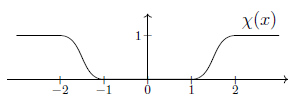
graphics grabbed from Dütsch 18, p. 108

and for ##\lambda \in (0,\infty)## a positive real number, write

$$
\chi_\lambda(x)
:=
\chi(\lambda x)
\,.
$$

Since the product ##\chi_\lambda u## has the support of a distribution on a complement of a neighbourhood of the origin, we may extend it by zero to distribution on all of ##\mathbb{R}^n##, which we will denote by the same symbols:

$$
\chi_\lambda u \in \mathcal{D}'(\mathbb{R}^n)
\,.
$$

By construction ##\chi_\lambda u## coincides with ##u## away from a neighbourhood of the origin, which moreover becomes arbitrarily small as ##\lambda## increases. This means that if the following limit exists

$$
\hat u
\;:=\;
\underset{\lambda \to \infty}{\lim}
\chi_\lambda u
$$

then it is an extension of ##u##.

To see that the limit exists, it is sufficient to observe that we have a Cauchy sequence, hence that for all ##b\in C^\infty_{cp}(\mathbb{R}^n)## the difference

$$
(\chi_{n+1} u – \chi_n u)(b)
\;=\;
u(b)( \chi_{n+1} + \chi_n )
$$

becomes arbitrarily small.

It remains to see that the unique extension ##\hat u## thus established has the same scaling degree as ##u##. This is shown in (Brunetti-Fredenhagen 00, p. 24).

Proposition 16.12. (space of point-extensions of distributions)

For ##n \in \mathbb{N}##, let ##u \in \mathcal{D}'(\mathbb{R}^n \setminus \{0\})## be a distribution of degree of divergence ##deg(u) \lt \infty##.

Then ##u## does admit at least one extension (def. 16.10) to a distribution ##\hat u \in \mathcal{D}'(\mathbb{R}^n)##, and every choice of extension has the same degree of divergence as ##u##

$$
deg(\hat u) = deg(u)
\,.
$$

Moreover, any two such extensions ##\hat u## and ##{\hat u}^\prime## differ by a linear combination of partial derivatives of distributions of order ##\leq deg(u)## of the delta distribution ##\delta_0## supported at the origin:

$$
{\hat u}^\prime
–
\hat u
\;=\;
\underset{
{ \alpha \in \mathbb{N}^n }
\atop
{ {\vert \alpha\vert} \leq deg(u) }
}{\sum}
q^\alpha
\partial_\alpha \delta_0
\,,
$$

for a finite number of constants ##q^\alpha \in \mathbb{C}##.

This is essentially (Hörmander 90, thm. 3.2.4). We follow (Brunetti-Fredenhagen 00, theorem 5.3), which was inspired by (Epstein-Glaser 73, section 5). Review of this approach is in (Dütsch 18, theorem 3.35 (b)), see also remark 16.13 below.

Proof. For ##f \in C^\infty(\mathbb{R}^n)## a smooth function, and ##\rho \in \mathbb{N}##, we say that ##f## vanishes to order ##\rho## at the origin if all partial derivatives with multi-index ##\alpha \in \mathbb{N}^n## of total order ##{\vert \alpha\vert} \leq \rho## vanish at the origin:

$$
\partial_\alpha f (0) = 0
\phantom{AAA}
{\vert \alpha\vert} \leq \rho
\,.
$$

By Hadamard’s lemma, such a function may be written in the form

$$
\label{ForVanishingOrderRhoHadamardExpansion}
f(x)
\;=\;
\underset{
{\alpha \in \mathbb{N}^n}
\atop
{ {\vert \alpha \vert} = \rho + 1 }
}{\sum}
x^\alpha
r_\alpha(x)
$$

(261)

for smooth functions ##r_\alpha \in C^\infty_{cp}(\mathbb{R}^n)##.

Write

$$
\mathcal{D}_\rho(\mathbb{R}^n)
\hookrightarrow
\mathcal{D}(\mathbb{R}^n)
:=
C^\infty_{cp}(\mathbb{R}^n)
$$

for the subspace of that of all bump functions on those that vanish to order ##\rho## at the origin.

By definition this is equivalently the joint kernel of the partial derivatives of distributions of order ##{\vert \alpha\vert}## of the delta distribution ##\delta_0## supported at the origin:

$$
b \in \mathcal{D}_\rho(\mathbb{R}^n)
\phantom{AA}
\Leftrightarrow
\phantom{AA}
\underset{
{\alpha \in \mathbb{N}^n}
\atop
{ {\vert \alpha\vert} \leq \rho }
}
{\forall}
\left\langle \partial_\alpha \delta_0, b \right\rangle
= 0
\,.
$$

Therefore every continuous linear projection

$$
\label{ForExtensionOfDistributionsProjectionMaps}
p_\rho
\;\colon\;
\mathcal{D}(\mathbb{R}^n)
\longrightarrow
\mathcal{D}_\rho(\mathbb{R}^n)
$$

(262)

maybe obtained from a choice of dual basis to the ##\{\partial_\alpha \delta_0\}##, hence a choice of smooth functions

$$
\left\{
w^\beta \in C^\infty_{cp}(\mathbb{R}^n)
\right\}_{ { \beta \in \mathbb{N}^n } \atop { {\vert \beta\vert} \leq \rho } }
$$

such that

$$
\left\langle
\partial_\alpha \delta_0
\,,\,
w^\beta
\right\rangle
\;=\;
\delta_\alpha^\beta
\phantom{AAA}
\Leftrightarrow
\phantom{AAA}
\partial_\alpha w^\beta(0)
\;=\;
\delta_\alpha^\beta
\phantom{AAAA}
\text{for}\, {\vert \alpha\vert} \leq \rho
\,,
$$

by setting

$$
\label{SpaceOfSmoothFunctionsOfGivenVaishingOrderProjector}
p_\rho
\;:=\;
id
\;-\;
\left\langle
\underset{
{\alpha \in \mathbb{N}^n}
\atop
{ {\vert \alpha\vert} \leq \rho }
}{\sum}
w^\alpha \partial_\alpha \delta_0
\,,\,
(-)
\right\rangle
\,,
$$

(263)

hence

$$
p_\rho
\;\colon\;
b
\mapsto
b
–
\underset{
{\alpha \in \mathbb{N}^n}
\atop
{ {\vert \alpha\vert} \leq \rho }
}{\sum}
(-1)^{{\vert \alpha\vert}} w^\alpha \partial_\alpha b(0)
\,.
$$

Together with Hadamard’s lemma in the form (261) this means that every ##b \in \mathcal{D}(\mathbb{R}^n)## is decomposed as

$$
\label{ForExtensionOfDistributionsTestFunctionDecomposition}
\begin{aligned}
b(x)
& =
p_\rho(b)(x)
\;+\;
(id – p_\rho)(b)(x)
\\
& =
\underset{
{ \alpha \in \mathbb{N}^n }
\atop
{ {\vert \alpha \vert} = \rho + 1 }
}{\sum}
x^\alpha r_\alpha(x)
\;+\;
\underset{
{ \alpha \in \mathbb{N}^n }
\atop
{ {\vert \alpha \vert} \leq \rho }
}{\sum}
(-1)^{{\vert \alpha \vert}}
w^\alpha \partial_\alpha b(0)
\end{aligned}
$$

(264)

Now let

$$
\rho
\;:=\;
deg(u)
\,.
$$

Observe that (by prop. 16.8) the degree of divergence of the product of distributions ##x^\alpha u## with ##{\vert \alpha\vert} = \rho + 1## is negative

$$
\begin{aligned}
deg\left(
x^\alpha u
\right)
& =
\rho – {\vert \alpha \vert}
\leq
-1
\end{aligned}
$$

Therefore prop. 16.11 says that each ##x^\alpha u## for ##{\vert \alpha\vert} = \rho + 1## has a unique extension ##\widehat{ x^\alpha u}## to the origin. Accordingly the composition ##u \circ p_\rho## has a unique extension, by (264):

$$
\label{ExtensionOfDitstributionsPointFixedAndChoice}
\begin{aligned}
\left\langle
\hat u
\,,\,
b
\right\rangle
& =
\left\langle
\hat u
,
p_\rho(b)
\right\rangle
+
\left\langle
\hat u
,
(id – p_\rho)(b)
\right\rangle
\\
& =
\underset{
{ \alpha \in \mathbb{N}^n }
\atop
{ {\vert \alpha \vert} = \rho + 1 }
}{\sum}
\underset{
\text{unique}
}{
\underbrace{
\left\langle
\widehat{x^\alpha u}
\,,\,
r_\alpha
\right\rangle
}
}
\;+\;
\underset{
{ \alpha \in \mathbb{N}^n }
\atop
{ {\vert \alpha\vert} \leq \rho }
}{\sum}
\underset{
{ q^\alpha }
\atop
{ \text{choice} }
}{
\underbrace{
\langle
\hat u
\,,\,
w^\alpha
\rangle
}
}
\left\langle
\partial_\alpha \delta_0
\,,\,
b
\right\rangle
\end{aligned}
$$

(265)

That says that ##\hat u## is of the form

$$
\hat u
\;=\;
\underset{
\text{unique}
}{
\underbrace{
\widehat{
u \circ p_\rho
}
}
}
+
\underset{
{ \alpha \in \mathbb{N}^n }
\atop
{ {\vert \alpha\vert} \leq \rho }
}{\sum}
c^\alpha
\,
\partial_\alpha \delta_0
$$

for a finite number of constants ##c^\alpha \in \mathbb{C}##.

Notice that for any extension ##\hat u## the exact value of the ##c^\alpha## here depends on the arbitrary choice of dual basis ##\{w^\alpha\}## used for this construction. But the uniqueness of the first summand means that for any two choices of extensions ##\hat u## and ##{\hat u}^\prime##, their difference is of the form

$$
{\hat u}^\prime – \hat u
\;=\;
\underset{
{ \alpha \in \mathbb{N}^n }
\atop
{ {\vert \alpha\vert} \leq \rho }
}{\sum}
( (c’)^\alpha – c^\alpha )
\,
\partial_\alpha \delta_0
\,,
$$

where the constants ##q^\alpha := ( (c’)^\alpha – c^\alpha ) \in \mathbb{C}## are independent of any choices.

It remains to see that all these ##\hat u## in fact have the same degree of divergence as ##u##.

By example 16.6 the degree of divergence of the point-supported distributions on the right is ##deg(\partial_\alpha \delta_0) = {\vert \alpha\vert} \leq \rho##.

Therefore to conclude it is now sufficient to show that

$$
deg\left(
\widehat{
u \circ p_\rho
}
\right)
\;=\;
\rho
\,.
$$

This is shown in (Brunetti-Fredenhagen 00, p. 25).

Remark 16.13. (“W-extensions”)

Since in Brunetti-Fredenhagen 00, (38) the projectors (263) are denoted “##W##”, the construction of extensions of distributions via the proof of prop. 16.12 has come to be called “W-extensions” (e.g Dütsch 18).

In conclusion we obtain the central theorem of causal perturbation theory:

Theorem 16.14. (existence and choices of (“re”-)normalization of S-matrices/perturbative QFTs)

Let ##(E_{\text{BV-BRST}}, \mathbf{L}’, \Delta_H )## be a gauge-fixed relativistic free vacuum, according to def. 15.1, such that the underlying spacetime is Minkowski spacetime and the Wightman propagator ##\Delta_H## is translation-invariant.

Then:

an S-matrix scheme ##\mathcal{S}## (def. 15.3) around this vacuum exists;
for ##g S_{int} + j A \in LocObs(E_{\text{BV-BRST}})[ [ \hbar, g, j] ]\langle g,j\rangle## a local observable as in def. 15.2, regarded as an adiabatically switched interaction action functional, the space of possible choices of S-matrices$$
\mathcal{S}(g S_{int} + j A)
\;\in\;
PolyObs(E_{\text{BV-BRST}})_{mc}[ [ \hbar, g, j] ]
$$hence of the corresponding perturbative QFTs, by prop. 15.25, is, inductively in ##k \in \mathbb{N}##, a finite dimensional affine space, parameterizing the extension of the time-ordered product ##T_k## to the locus of coinciding interaction points.

Proof. By prop. 16.7 the Feynman propagator is finite scaling degree of a distribution, so that by prop. 16.9 the binary time-ordered product away from the diagonal ##T_2(-,-)\vert_{\Sigma^2 \setminus diag(\Sigma)} = (-) \star_{F} (-)## has finite scaling degree.

By prop. 16.9 this implies that in the inductive description of the time-ordered products by prop. 16.1, each induction step is the extension of distributions of finite scaling degree of a distribution to the point. By prop. 16.12 this always exists.

This proves the first statement.

Now if a polynomial local interaction is fixed, then via remark 16.2
each induction step involved extending a finite number of distributions, each of finite scaling degree. By prop. 16.12 the corresponding space of choices is in each step a finite-dimensional affine space.

Stückelberg-Petermann renormalization group

A genuine re-normalization is the passage from one S-matrix (“re”-)normalization scheme ##\mathcal{S}## to another such scheme ##\mathcal{S}’##. The inductive Epstein-Glaser (“re”-normalization) construction (prop. 16.1) shows that the difference between any ##\mathcal{S}## and ##\mathcal{S}’## is inductively in ##k \in \mathbb{N}## a choice of extra term in the time-ordered product of ##k## factors, equivalently in the Feynman amplitudes for Feynman diagrams with ##k## vertices, that contributes when all ##k## of these vertices coincide in spacetime (prop. 16.12).

A natural question is whether these additional interactions that appear when several interaction vertices coincide may be absorbed into a re-definition of the original interaction ##g S_{int} + j A##. Such an interaction vertex redefinition (def. 16.15 below)

$$
\mathcal{Z}
\;\colon\;
g S_{int} + j A
\;\mapsto\;
g S_{int} + j A
\;+\;
\text{higher order corrections}
$$

should perturbatively send local interactions to local interactions with higher-order corrections.

The main theorem of perturbative renormalization (theorem 16.19 below) says that indeed under mild conditions every re-normalization ##\mathcal{S} \mapsto \mathcal{S}’## is induced by such an interaction vertex redefinition in that there exists a unique such redefinition ##\mathcal{Z}## so that for every local interaction ##g S_{int} + j A## we have that scattering amplitudes for the interaction ##g S_{int} + j A## computed with the (“re”-)normalization scheme ##\mathcal{S}’## equal those computed with ##\mathcal{S}## but applied to the re-defined interaction ##\mathcal{Z}(g S_{int} + j A)##:

$$
\mathcal{S}’
\left(
{\, \atop \,}
g S_{int} + j A
{\, \atop \,}
\right)
\;=\;
\mathcal{S}\left( {\, \atop \,} \mathcal{Z}(g S_{int} + j A) {\, \atop \,} \right)
\,.
$$

This means that the interaction vertex redefinitions ##\mathcal{Z}## form a group under composition which acts transitively and freely, hence regularly, on the set of S-matrix (“re”-)normalization schemes; this is called the Stückelberg-Petermann renormalization group (theorem 16.19 below).

Definition 16.15. (perturbative interaction vertex redefinition)

Let ##(E_{\text{BV-BRST}}, \mathbf{L}’, \Delta_H)## be a gauge fixed free field vacuum (def. 15.1).

A perturbative interaction vertex redefinition (or just vertex redefinition, for short) is an endofunction

$$
\mathcal{Z}
\;\colon\;
LocObs(E_{\text{BV-BRST}})[ [ \hbar, g, j] ]\langle g, j\rangle
\longrightarrow
LocObs(E_{\text{BV-BRST}})[ [ \hbar, g, j] ]\langle g, j\rangle
$$

on local observables with formal parameters adjoined (def. 15.2) such that there exists a sequence ##\{Z_k\}_{k \in \mathbb{N}}## of continuous linear functionals, symmetric in their arguments, of the form

$$
\left(
{\, \atop \,}
LocObs(E_{\text{BV-BRST}})[ [ \hbar, g, j] ]\langle g, j\rangle
{\, \atop \,}
\right)^{\otimes^k_{\mathbb{C}[ [ \hbar, g, j] ]}}
\longrightarrow
LocObs(E_{\text{BV-BRST}})[ [ \hbar, g, j] ]\langle g, j\rangle
$$

such that for all ##g S_{int} + j A \in LocObs(E_{\text{BV-BRST}})[ [ \hbar, g, j] ]\langle g, j\rangle## the following conditions hold:

(perturbation)
1. ##Z_0(g S_{int + j A}) = 0##
2. ##Z_1(g S_{int} + j A) = g S_{int} + j A##
3. and$$
  \begin{aligned}
  \mathcal{Z}(g S_{int} + j A)
  & =
  Z \exp_\otimes( g S_{int} + j A )
  \\
  &
  :=
  \underset{k \in \mathbb{N}}{\sum}
  \frac{1}{k!}
  Z_k(
  \underset{
  k \, \text{args}
  }{
  \underbrace{
  g S_{int} + j A , \cdots, g S_{int} + j A
  }
  }
  )
  \end{aligned}
  $$

(field independence) The local observable ##\mathcal{Z}(g S_{int} + j A)## depends on the field histories only through its argument ##g S_{int} + j A ##, hence by the chain rule:

$$
\label{FieldIndependenceVertexRedefinition}
\frac{\delta}{\delta \mathbf{\Phi}^a(x)}
\mathcal{Z}(g S_{int} + j A)
\;=\;
\mathcal{Z}’_{g S_{int} + j A}
\left(
\frac{\delta}{\delta \mathbf{\Phi}^a(x)} (g S_{int} + j A)
\right)
$$

(266)

The following proposition should be compared to the axiom of causal additivity of the S-matrix scheme (228):

Proposition 16.16. (local additivity of vertex redefinitions)

Let ##(E_{\text{BV-BRST}}, \mathbf{L}’, \Delta_H)## be a gauge fixed free field vacuum (def. 15.1) and let ##\mathcal{Z}## be a vertex redefinition (def. 16.15).

Then for all local observables ##O_0, O_1, O_2 \in LocObs(E_{\text{BV-BRST}})[ [ \hbar, g, j ] ]\langle g, j\rangle## with spacetime support denoted ##supp(O_i) \subset \Sigma## (def. 7.31) we have

(local additivity)$$
\begin{aligned}
&
\left(
supp(O_1)
\cap
supp(O_2)
=
\emptyset
\right)
\\
&
\Rightarrow
\phantom{AA}
\mathcal{Z}( O_0 + O_1 + O_2)
=
\mathcal{Z}( O_0 + O_1 ) – \mathcal{Z}(O_0) + \mathcal{Z}(O_0 + O_2)
\end{aligned}
\,.
$$
(preservation of spacetime support)$$
supp
\left(
{\, \atop \,}
\mathcal{Z}(O_0 + O_1)
–
\mathcal{Z}(O_0)
{\, \atop \,}
\right)
\;\subset\;
supp(O_1)
$$hence in particular$$
supp
\left(
{\, \atop \,}
\mathcal{Z}(O_1)
{\, \atop \,}
\right) = supp(O_1)
$$

(Dütsch 18, exercise 3.98)

Proof. Under the inclusion

$$
LocObs(E_{\text{BV-BRST}})
\hookrightarrow
PolyObs(E_{\text{BV-BRST}})
$$

of local observables into polynomial observables, we may think of each ##Z_k## as a generalized function, as for time-ordered products in remark 15.33.

Hence if

$$
O_j = \underset{\Sigma}{\int} j^\infty_\Sigma( \mathbf{L}_j )
$$

is the transgression of a Lagrangian density ##\mathbf{L}## we get

$$
Z_k(
(O_1 + O_2 + O_3)
,
\cdots
,
(O_1 + O_2 + O_3)
)
=
\underset{
j_1, \cdots, j_k \in \{0,1,2\}
}{\sum}
\underset{\Sigma^{k}}{\int}
Z( \mathbf{L}_{j_1}(x_1) , \cdots , \mathbf{L}_{j_k}(x_k) )
\,.
$$

Now by definition ##Z_k(\cdots)## is in the subspace of local observables, i.e. those polynomial observables whose coefficient distributions are supported on the diagonal, which means that

$$
\frac{\delta}{\delta \mathbf{\Phi}^a(x)}
\frac{\delta}{\delta \mathbf{\Phi}^b(y)}
Z_{k}(\cdots)
=
0
\phantom{AA}
\text{for}
\phantom{AA}
x \neq y
$$

Together with the axiom “field independence” (266) this means that the support of these generalized functions in the integrand here must be on the diagonal, where ##x_1 = \cdots = x_k##.

By the assumption that the spacetime supports of ##O_1## and ##O_2## are disjoint, this means that only the summands with ##j_1, \cdots, j_k \in \{0,1\}## and those with ##j_1, \cdots, j_k \in \{0,2\}## contribute to the above sum. Removing the overcounting of those summands where all ##j_1, \cdots, j_k \in \{0\}## we get

$$
\begin{aligned}
& Z_k\left(
{\, \atop \,}
(O_1 + O_2 + O_3)
,
\cdots
,
(O_1 + O_2 + O_3)
{\, \atop \,}
\right)
\\
& =
\underset{
j_1, \cdots, j_k \in \{0,1\}
}{\sum}
\underset{\Sigma^{k}}{\int}
Z( \mathbf{L}_{j_1}(x_1) , \cdots , \mathbf{L}_{j_k}(x_k) )
\\
& \phantom{=}
–
\underset{
j_1, \cdots, j_k \in \{0\}
}{\sum}
\underset{\Sigma^{k}}{\int}
Z( \mathbf{L}_{j_1}(x_1) , \cdots , \mathbf{L}_{j_k}(x_k) )
\\
& \phantom{=}
–
\underset{
j_1, \cdots, j_k \in \{0,2\}
}{\sum}
\underset{\Sigma^{k}}{\int}
Z( \mathbf{L}_{j_1}(x_1) , \cdots , \mathbf{L}_{j_k}(x_k) )
\\
& =
Z_k\left( {\, \atop \,} (O_0 + O_1), \cdots, (O_0 + O_1) {\, \atop \,}\right)
–
Z_k\left( {\, \atop \,} O_0, \cdots, O_0 {\, \atop \,} \right)
+
Z_k\left( {\, \atop \,} (O_0 + O_2), \cdots, (O_0 + O_2) {\, \atop \,} \right)
\end{aligned}
\,.
$$

This directly implies the claim.

As a corollary we obtain:

Proposition 16.17. (composition of S-matrix scheme with vertex redefinition is again S-matrix scheme)

Let ##(E_{\text{BV-BRST}}, \mathbf{L}’, \Delta_H)## be a gauge fixed free field vacuum (def. 15.1) and let ##\mathcal{Z}## be a vertex redefinition (def. 16.15).

Then for

$$
\mathcal{S}
\;\colon\;
LocObs(E_{\text{BV-BRST}})[ [ \hbar, g, j] ]\langle g, j\rangle
\longrightarrow
PolyObs(E_{\text{BV-BRST}})_{mc}((\hbar))[ [ g,j ] ]
$$

and S-matrix scheme (def. 15.3), the composite

$$
\mathcal{S} \circ \mathcal{Z}
\;\colon\;
LocObs(E_{\text{BV-BRST}})[ [ \hbar, g, j] ]\langle g, j\rangle
\overset{\mathcal{Z}}{\longrightarrow}
LocObs(E_{\text{BV-BRST}})[ [ \hbar, g, j] ]\langle g, j\rangle
\overset{\mathcal{S}}{\longrightarrow}
PolyObs(E_{\text{BV-BRST}})_{mc}((\hbar))[ [ g,j ] ]
$$

is again an S-matrix scheme.

Moreover, if ##\mathcal{S}## satisfies the renormalization condition “field independence” (prop. 15.49), then so does ##\mathcal{S} \circ \mathcal{Z}##.

(e.g Dütsch 18, theorem 3.99 (b))

Proof. It is clear that the causal order of the spacetime supports implies that they are in particular disjoint

$$
\left(
{\, \atop \,}
supp(O_1)
{\vee\!\!\!\wedge}
supp(O_2)
{\, \atop \,}
\right)
\phantom{AA}
\Rightarrow
\phantom{AA}
\left(
{\, \atop \,}
supp(O_1)
\cap
supp(O_)
\;=\;
\emptyset
{\, \atop \,}
\right)
$$

Therefore the local additivity of ##\mathcal{Z}## (prop. 16.16) and the causal factorization of the S-matrix (remark 15.15) imply the causal factorization of the composite:

$$
\begin{aligned}
\mathcal{S}
\left(
{\, \atop \,}
\mathcal{Z}(O_1 + O_2)
{\, \atop \,}
\right)
& =
\mathcal{S}
\left(
{\, \atop \,}
\mathcal{Z}(O_1)
+
\mathcal{Z}(O_2)
{\, \atop \,}
\right)
\\
& =
\mathcal{S}
\left(
{\, \atop \,}
\mathcal{Z}(O_1)
{\, \atop \,}
\right)
\,
\mathcal{S}
\left(
{\, \atop \,}
\mathcal{Z}(O_2)
{\, \atop \,}
\right)
\,.
\end{aligned}
$$

But by prop. 15.40 this implies, in turn, causal additivity and hence that ##\mathcal{S} \circ \mathcal{Z}## is itself an S-matrix scheme.

Finally that ##\mathcal{S} \circ \mathcal{Z}## satisfies “field indepndence” if ##\mathcal{S}## does is immediate by the chain rule, given that ##\mathcal{Z}## satisfies this condition by definition.

Proposition 16.18. (any two S-matrix renormalization schemes differ by unique vertex redefinition)

Let ##(E_{\text{BV-BRST}}, \mathbf{L}’, \Delta_H)## be a gauge fixed free field vacuum (def. 15.1).

Then for ##\mathcal{S}, \mathcal{S}’## any two S-matrix schemes (def. 15.3) which both satisfy the renormalization condition “field independence”, the there exists a unique vertex redefinition ##\mathcal{Z}## (def. 16.15) relating them by composition, i. e. such that

$$
\mathcal{S}’
\;=\;
\mathcal{S} \circ \mathcal{Z}
\,.
$$

Proof. By applying both sides of the equation to linear combinations of local observables of the form ##\kappa_1 O_1 + \cdots + \kappa_k O_k## and then taking derivSatives with respect to ##\kappa## at ##\kappa_j = 0## (as in example 15.32) we get that the equation in question implies

$$
(i \hbar)^k
\frac{
\partial^k
}{
\partial \kappa_1 \cdots \partial \kappa_k
}
\mathcal{S}'( \kappa_1 O_1 + \cdots + \kappa_k O_k )
\vert_{\kappa_1, \cdots, \kappa_k = 0}
\;=\;
(i \hbar)^k
\frac{
\partial^k
}{
\partial \kappa_1 \cdots \partial \kappa_k
}
\mathcal{S} \circ \mathcal{Z}( \kappa_1 O_1 + \cdots + \kappa_k O_k )
\vert_{\kappa_1, \cdots, \kappa_k = 0}
$$

which in components means that

$$
\begin{aligned}
T’_k( O_1, \cdots, O_k )
& =
\underset{
2 \leq n \leq k
}{\sum}
\frac{1}{n!}
(i \hbar)^{k-n}
\underset{
{ { I_1 \sqcup \cdots \sqcup I_n } \atop { = \{1, \cdots, k\}, } }
\atop
{ I_1, \cdots, I_n \neq \emptyset }
}{\sum}
T_n
\left(
{\, \atop \,}
Z_{{\vert I_1\vert}}\left( (O_{i_1})_{i_1 \in I_1} \right),
\cdots,
Z_{{\vert I_n\vert}}\left( (O_{i_n})_{i_n \in I_n} \right),
{\, \atop \,}
\right)
\\
& \phantom{=}
+
Z_k( O_1,\cdots, O_k )
\end{aligned}
$$

where ##\{T’_k\}_{k \in \mathbb{N}}## are the time-ordered products corresponding to ##\mathcal{S}’## (by example 15.32) and ##\{T_k\}_{k \in \mathcal{N}}## those correspondong to ##\mathcal{S}##.

Here the sum on the right runs over all ways that in the composite ##\mathcal{S} \circ \mathcal{Z}## a ##k##-ary operation arises as the composite of an ##n##-ary time-ordered product applied to the ##{\vert I_i\vert}##-ary components of ##\mathcal{Z}##, for ##i## running from 1 to ##n##; except for the case ##k = n##, which is displayed separately in the second line

This shows that if ##\mathcal{Z}## exists, then it is unique because its coefficients ##Z_k## are inductively in ##k## given by the expressions

$$
\label{MainTheoremPerturbativeRenormalizationInductionStep}
\begin{aligned}
& Z_k( O_1,\cdots, O_k )
\\
& =
T’_k( O_1, \cdots, O_k )
\;-\;
\underset{
(T \circ \mathcal{Z}_{\lt k})_k
}{
\underbrace{
\underset{
2 \leq n \leq k
}{\sum}
\frac{1}{n!}
(i \hbar)^{k-n}
\underset{
{ { I_1 \sqcup \cdots \sqcup I_n } \atop { = \{1, \cdots, k\}, } }
\atop
{ I_1, \cdots, I_n \neq \emptyset }
}{\sum}
T_n
\left(
Z_{{\vert I_1\vert}}( (O_{i_1})_{i_1 \in I_1} ),
\cdots,
Z_{{\vert I_n\vert}}( (O_{i_n})_{i_n \in I_n} ),
\right)
}
}
\end{aligned}
$$

(267)

(The symbol under the brace is introduced as a convenient shorthand for the term above the brace.)

Hence it remains to see that the ##Z_k## defined this way satisfy the conditions in def. 16.15.

The condition “perturbation” is immediate from the corresponding condition on ##\mathcal{S}## and ##\mathcal{S}’##.

Similarly the condition “field independence” follows immediately from the assumoption that ##\mathcal{S}## and ##\mathcal{S}’## satisfy this condition.

It only remains to see that ##Z_k## indeed takes values in local observables. Given that the time-ordered products a priori take values in the larger space of microcausal polynomial observables this means to show that the spacetime support of ##Z_k## is on the diagonal.

But observe that, as indicated in the above formula, the term over the brace may be understood as the coefficient at order ##k## of the exponential series-expansion of the composite ##\mathcal{S} \circ \mathcal{Z}_{\lt k}##, where

$$
\mathcal{Z}_{\lt k}
\;:=\;
\underset{
n \in \{1, \cdots, k-1\}
}{\sum}
\frac{1}{n!} Z_n
$$

is the truncation of the vertex redefinition to degree ##\lt k##. This truncation is clearly itself still a vertex redefinition (according to def. 16.15) so that the composite ##\mathcal{S} \circ \mathcal{Z}_{\lt k}## is still an S-matrix scheme (by prop. 16.17) so that the ##(T \circ \mathcal{Z}_{\lt k})_k## are time-ordered products (by example 15.32).

So as we solve ##\mathcal{S}’ = \mathcal{S} \circ \mathcal{Z}## inductively in degree ##k##, then for the induction step in degree ##k## the expressions ##T’_{\lt k}## and ##(T \circ \mathcal{Z})_{\lt k}## agree and are both time-ordered products. By prop. 16.1 this implies that ##T’_{k}## and ##(T \circ \mathcal{Z}_{\lt k})_{k}## agree away from the diagonal. This means that their difference ##Z_k## is supported on the diagonal, and hence is indeed local.

In conclusion this establishes the following pivotal statement of perturbative quantum field theory:

Theorem 16.19. (main theorem of perturbative renormalization — Stückelberg-Petermann renormalization group of vertex redefinitions)

Let ##(E_{\text{BV-BRST}}, \mathbf{L}’, \Delta_H)## be a gauge fixed free field vacuum (def. 15.1).

the vertex redefinitions ##\mathcal{Z}## (def. 16.15) form a group under composition;
the set of S-matrix (“re”-)normalization schemes (def. 15.3), remark 15.22) satisfying the renormalization condition “field independence” (prop. 15.49) is a torsor over this group, hence equipped with a regular action in that
1. the set of S-matrix schemes is non-empty;
2. any two S-matrix (“re”-)normalization schemes ##\mathcal{S}##, ##\mathcal{S}’## are related by a unique vertex redefinition ##\mathcal{Z}## via composition:$$
  \mathcal{S}’ \;=\; \mathcal{S} \circ \mathcal{Z}
  \,.
  $$

This group is called the Stückelberg-Petermann renormalization group.

Typically one imposes a set of renormalization conditions (def. 15.48) and considers the corresponding subgroup of vertex redefinitions preserving these conditions.

Proof. The group structure and regular action are given by prop. 16.17 and prop. 16.18. The existence of S-matrices follows is the statement of Epstein-Glaser (“re”-)normalization in theorem 16.14.

UV-Regularization via counterterms

While Epstein-Glaser renormalization (prop. 16.1) gives a transparent picture of the space of choices in (“re”-)normalization (theorem 16.14) the physical nature of the higher interactions that it introduces at coincident interaction points (via the extensions of distributions in prop. 16.12) remains more implicit. But the main theorem of perturbative renormalization (theorem 16.19), which re-expresses the difference between any two such choices as an interaction vertex redefinition, suggests that already the choice of (“re”-)normalization itself should have an incarnation in terms of interaction vertex redefinitions.

This may be realized via a construction of (“re”-)normalization in terms of UV-regularization (prop. 16.23 below): For any choice of “UV-cutoff”, given by an approximation of the Feynman propagator ##\Delta_F## by non-singular distributions ##\Delta_{F,\Lambda}## (def. 16.20 below) there is a unique “effective S-matrix” ##\mathcal{S}_\Lambda## induced at each cutoff scale (def. 16.22 below). While the “UV-limit” ##\underset{\Lambda \to \infty}{\lim} \mathcal{S}_\Lambda## does not in general exist, it may be “regularized” by applying suitable interaction vertex redefinitions ##\mathcal{Z}_\Lambda##; if the higher-order corrections that these introduce serve to “counter” (remark 16.24 below) the coresponding UV-divergences.

This perspective of (“re”-)normalization via counterterms is often regarded as the primary one. Its elegant proof in prop. 16.23 below, however, relies on the Epstein-Glaser renormalization via inductive extensions of distributions and uses the same kind of argument as in the proof of the main theorem of perturbative renormalization (theorem 16.19 via prop. 16.18) that establishes the Stückelberg-Petermann renormalization group.

Definition 16.20. (UV cutoffs)

Let ##(E_{\text{BV-BRST}}, \mathbf{L}’, \Delta_H )## be a gauge fixed relativistic free vacuum over Minkowski spacetime ##\Sigma## (according to def. 15.1), where ##\Delta_H = \tfrac{i}{2}(\Delta_+ – \Delta_-) + H## is the corresponding Wightman propagator inducing the Feynman propagator

$$
\Delta_F \in \Gamma’_{\Sigma \times \Sigma}(E_{\text{BV-BRST}} \boxtimes E_{\text{BV-BRST}})
$$

by ##\Delta_F = \tfrac{i}{2}(\Delta_+ + \Delta_-) + H##.

Then a choice of UV cutoffs for perturbative QFT around this vacuum is a collection of non-singular distributions ##\Delta_{F,\Lambda}## parameterized by positive real numbers

$$
\array{
(0, \infty)
&\overset{}{\longrightarrow}&
\Gamma_{\Sigma \times \Sigma,cp}(E_{\text{BV-BRST}} \boxtimes E_{\text{BV-BRST}})
\\
\Lambda &\mapsto& \Delta_{F,\Lambda}
}
$$

such that:

each ##\Delta_{F,\Lambda}## satisfies the following basic properties
1. (translation invariance)$$
  \Delta_{F,\Lambda}(x,y) = \Delta_{F,\Lambda}(x-y)
  $$
2. (symmetry)$$
  \Delta^{b a}_{F,\Lambda}(y, x)
  \;=\;
  \Delta^{a b}_{F,\Lambda}(x, y)
  $$i.e.$$
  \Delta_{F,\Lambda}^{b a}(-x)
  \;=\;
  \Delta_{F,\Lambda}^{a b}(x)
  $$
the ##\Delta_{F,\Lambda}## interpolate between zero and the Feynman propagator, in that, in the Hörmander topology:
1. the limit as ##\Lambda \to 0## exists and is zero$$
  \underset{\Lambda \to \infty}{\lim} \Delta_{F,\Lambda}
  \;=\;
  0
  \,.
  $$
2. the limit as ##\Lambda \to \infty## exists and is the Feynman propagator:$$
  \underset{\Lambda \to \infty}{\lim} \Delta_{F,\Lambda}
  \;=\;
  \Delta_F
  \,.
  $$

(Dütsch 10, section 4)

Example 16.21. (relativistic momentum cutoff)

Recall from this prop. that the Fourier transform of distributions of the Feynman propagator for the real scalar field on Minkowski spacetime ##\mathbb{R}^{p,1}## is,

$$
\begin{aligned}
\widehat{\Delta}_F(k)
& =
\frac{+i}{(2\pi)^{p+1}}
\frac{
1
}{
– \eta(k,k) – \left( \tfrac{m c}{\hbar} \right)^2 + i 0
}
\end{aligned}
$$

To produce a UV cutoff in the sense of def. 16.20 we would like to set this function to zero for wave numbers ##\vert \vec k\vert## (hence momenta ##\hbar\vert \vec k\vert##) larger than a given ##\Lambda##.

This needs to be done with due care: First, the Paley-Wiener-Schwartz theorem (prop. 9.19) says that ##\Delta_{F,\Lambda}## to be a test function and hence compactly supported, its Fourier transform ##\widehat{\Delta}_{F,\Lambda}## needs to be smooth and of bounded growth. So instead of multiplying ##\widehat{\Delta}_F## by a step function in ##k##, we may multiply it with exponential damping.

(Keller-Kopper-Schophaus 97, section 6.1, Dütsch 18, example 3.126)

Definition 16.22. (effective S-matrix scheme)

Let ##(E_{\text{BV-BRST}}, \mathbf{L}’, \Delta_H )## be a gauge fixed relativistic free vacuum (according to def. 15.1) and let ##\left\{ \Delta_{F,\Lambda}\right\}_{\Lambda \in [0,\infty)}## be a choice of UV cutoffs for perturbative QFT around this vacuum (def. 16.20).

We say that the effective S-matrix scheme ##\mathcal{S}_\Lambda## at cutoff scale ##\Lambda \in [0,\infty)##

$$
\array{
PolyObs(E_{\text{BV-BRST}})_{mc}[ [ \hbar, g, j] ]
&\overset{\mathcal{S}_{\Lambda}}{\longrightarrow}&
PolyObs(E_{\text{BV-BRST}})_{mc}[ [ \hbar, g, j] ]
\\
O &\mapsto& \mathcal{S}_\Lambda(O)
}
$$

is the exponential series

$$
\label{EffectiveSMatrixScheme}
\begin{aligned}
\mathcal{S}_\Lambda(O)
& :=
\exp_{F,\Lambda}\left( \frac{1}{i \hbar} O \right)
\\
& =
1
+
\frac{1}{i \hbar} O
+
\frac{1}{2} \frac{1}{(i \hbar)^2} O \star_{F,\Lambda} O
+
\frac{1}{3!} \frac{1}{(i \hbar)^3} O \star_{F,\Lambda} O \star_{F,\Lambda} 0
+
\cdots
\end{aligned}
\,.
$$

(268)

with respect to the star product ##\star_{F,\Lambda}## induced by the ##\Delta_{F,\Lambda}## (def. 13.18).

This is evidently defined on all polynomial observables as shown and restricts to an endomorphism on microcausal polynomial observables as shown, since the contraction coefficients ##\Delta_{F,\Lambda}## are non-singular distributions, by definition of UV cutoff.

(Dütsch 10, (4.2))

Proposition 16.23. ((“re”-)normalization via UV regularization)

Let ##(E_{\text{BV-BRST}}, \mathbf{L}’, \Delta_H )## be a gauge fixed relativistic free vacuum (according to def. 15.1) and let ##g S_{int} + j A \in LocObs(E_{\text{BV-BRST}})[ [ \hbar, g, j] ]\langle g,j\rangle## a polynomial local observable as in def. 15.2, regarded as an adiabatically switched interaction action functional.

Let moreover ##\{\Delta_{F,\Lambda}\}_{\Lambda \in [0,\infty)}## be a UV cutoff (def. 16.20); with ##\mathcal{S}_\Lambda## the induced effective S-matrix schemes (268).

Then

there exists a ##[0,\infty)##-parameterized interaction vertex redefinition ##\{\mathcal{Z}_\Lambda\}_{\Lambda \in \mathbb{R}_{\geq 0}}## (def. 16.15) such that the limit of effective S-matrix schemes ##\mathcal{S}_{\Lambda}## (268) applied to the ##\mathcal{Z}_\Lambda##-redefined interactions$$
\mathcal{S}_\infty
\;:=\;
\underset{\Lambda \to \infty}{\lim}
\left(
\mathcal{S}_\Lambda \circ \mathcal{Z}_\Lambda
\right)
$$exists and is a genuine S-matrix scheme around the given vacuum (def. 15.3);
every S-matrix scheme around the given vacuum arises this way.

These ##\mathcal{Z}_\Lambda## are called counterterms (remark 16.24 below) and the composite ##\mathcal{S}_\Lambda \circ \mathcal{Z}_\Lambda## is called a UV regularization of the effective S-matrices ##\mathcal{S}_\Lambda##.

Hence UV-regularization via counterterms is a method of (“re”-)normalization of perturbative QFT (def. 15.46).

This was claimed in (Brunetti-Dütsch-Fredenhagen 09, (75)), a proof was indicated in (Dütsch-Fredenhagen-Keller-Rejzner 14, theorem A.1).

Proof. Let ##\{p_{\rho_{k}}\}_{k \in \mathbb{N}}## be a sequence of projection maps as in (262) defining an Epstein-Glaser (“re”-)normalization (prop. 16.1) of time-ordered products ##\{T_k\}_{k \in \mathbb{N}}## as extensions of distributions of the ##T_k##, regarded as distributions via remark 16.2, by the choice ##q_k^\alpha = 0## in (265).

We will construct that ##\mathcal{Z}_\Lambda## in terms of these projections ##p_\rho##.

First, consider some convenient shorthand:

For ##n \in \mathbb{N}##, write ##\mathcal{Z}_{\leq n} := \underset{1 \in \{1, \cdots, n\}}{\sum} \frac{1}{n!} Z_n##. Moreover, for ##k \in \mathbb{N}## write ##(T_\Lambda \circ \mathcal{Z}_{\leq n})_k## for the ##k##-ary coefficient in the expansion of the composite ##\mathcal{S}_\Lambda \circ \mathcal{Z}_{\leq n}##, as in equation (267) in the proof of the main theorem of perturbative renormalization (theorem 16.19, via prop. 16.18).

In this notation, we need to find ##\mathcal{Z}_\Lambda## such that for each ##n \in \mathbb{N}## we have

$$
\label{CountertermsInductionAssumption}
\underset{\Lambda \to \infty}{\lim}
\left(
T_\Lambda \circ \mathcal{Z}_{\leq n, \Lambda}
\right)_n
\;=\;
T_n
\,.
$$

(269)

We proceed by induction over ##n \in \mathbb{N}##.

Since by definition ##T_0 = const_1##, ##T_1 = id## and ##Z_0 = const_0##, ##Z_1 = id## the statement is trivially true for ##n = 0## and ##n = 1##.

So assume now ##n \in \mathbb{N}## and ##\{Z_{k}\}_{k \leq n}## has been found such that (269) holds.

Observe that with the chosen renormalizing projection ##p_{\rho_{n+1}}## the time-ordered product ##T_{n+1}## may be expressed as follows:

$$
\label{RenormalizedSMatrixAsLimitOfEffectiveSMatricesEvaluatedOnProjection}
\begin{aligned}
T_{n+1}(O, \cdots, O)
& =
\left\langle
\underset{ {\mathbf{I} \in \{1, \cdots, n+1\} } \atop { \mathbf{I}, \overline{\mathbf{I}} \neq \emptyset } }{\sum}
\!\!\chi_i(\mathbf{X})\,
\left(
{\, \atop \,}
T_{{\vert \mathbf{I}\vert}} (\mathbf{I})
{\, \atop \,}
\right)
\star_{F}
\left(
{\, \atop \,}
T_{ {\vert \overline{\mathbf{I}} \vert} } ( \overline{\mathbf{I}} )
{\, \atop \,}
\right)
\,,\,
p_{\rho_k}(O \otimes \cdots \otimes O)
\right\rangle
\\
& =
\left\langle
\underset{\Lambda \to \infty}{\lim}
\underset{ {\mathbf{I} \in \{1, \cdots, n+1\} } \atop { \mathbf{I}, \overline{\mathbf{I}} \neq \emptyset } }{\sum}
\!\!\chi_i(\mathbf{X})\,
\left(
{\, \atop \,}
T_{{\vert \mathbf{I}\vert}} (\mathbf{I})
{\, \atop \,}
\right)
\star_{F,\Lambda}
\left(
{\, \atop \,}
T_{ {\vert \overline{\mathbf{I}} \vert} } ( \overline{\mathbf{I}} )
{\, \atop \,}
\right)
\,,\,
p_{\rho_k}(O \otimes \cdots \otimes O)
\right\rangle
\end{aligned}
\,.
$$

(270)

Here in the first step, we inserted the causal decomposition (260) of ##T_{n+1}## in terms of the ##\{T_k\}_{k \leq n}## away from the diagonal, as in the proof of prop. 16.1, which is admissible because the image of ##p_{\rho_{n+1}}## vanishes on the diagonal. In the second step we replaced the star-product of the Feynman propagator ##\Delta_F## with the limit over the star-products of the regularized propagators ##\Delta_{F,\Lambda}##, which converges by the nature of the Hörmander topology (which is assumed by def. 16.20).

Hence it is sufficient to find ##Z_{n+1,\Lambda}## and ##K_{n+1,\Lambda}## such that

$$
\label{CountertermsAndCorrectionTerm}
\begin{aligned}
\left\langle
\left(
T_{\Lambda} \circ \mathcal{Z}_{\Lambda}
\right)_{n+1}
\,,\,
(-, \cdots, -)
\right\rangle
& =
\left\langle
\underset{ {\mathbf{I} \in \{1, \cdots, n+1\} } \atop { \mathbf{I}, \overline{\mathbf{I}} \neq \emptyset } }{\sum}
\!\!\chi_i(\mathbf{X})\,
\left(
{\, \atop \,}
T_{{\vert \mathbf{I}\vert}} (\mathbf{I})
{\, \atop \,}
\right)
\star_{F,\Lambda}
\left(
{\, \atop \,}
T_{ {\vert \overline{\mathbf{I}} \vert} } ( \overline{\mathbf{I}} )
{\, \atop \,}
\right)
\,,\,
p_{\rho_{k}}\left( -, \cdots, – \right)
\right\rangle
\\
& \phantom{=}
+
K_{n+1,\Lambda}(-, \cdots, -)
\end{aligned}
$$

(271)

subject to these two conditions:

##\mathcal{Z}_{n+1,\Lambda}## is local;
##\underset{\Lambda \to \infty}{\lim} K_{n+1,\Lambda} = 0##.

Now by expanding out the left hand side of (271) as

$$
(T_\Lambda \circ \mathcal{Z}_\Lambda)_{n+1}
\;=\;
Z_{n+1,\Lambda}
\;+\;
(T_\Lambda \circ Z_{\leq n, \Lambda})_{n+1}
$$

(which uses the condition ##T_1 = id##) we find the unique solution of (271) for ##Z_{n+1,\Lambda}##, in terms of the ##\{Z_{\leq n,\Lambda}\}## and ##K_{n+1,\Lambda}## (the latter still to be chosen) to be:

$$
\label{CountertermOrderByOrderInTermsOfCorrectionTerm}
\begin{aligned}
\left\langle
Z_{n+1,\Lambda}
,
(-,\cdots, -)
\right\rangle
& =
\left\langle
\underset{ {\mathbf{I} \in \{1, \cdots, n+1\} } \atop { \mathbf{I}, \overline{\mathbf{I}} \neq \emptyset } }{\sum}
\!\!\chi_i(\mathbf{X})\,
\left(
{\, \atop \,}
T_{{\vert \mathbf{I}\vert}} (\mathbf{I})
{\, \atop \,}
\right)
\star_{F,\Lambda}
\left(
{\, \atop \,}
T_{ {\vert \overline{\mathbf{I}} \vert} } ( \overline{\mathbf{I}} )
{\, \atop \,}
\right)
\,,\,
p_{\rho_{n+1}}(-, \cdots, -)
\right\rangle
\\
& \phantom{=}
–
\left\langle
\left(
T_{\Lambda} \circ \mathcal{Z}_{\leq n,\Lambda}
\right)_{n+1}
\,,\,
(-, \cdots, -)
\right\rangle
\\
& \phantom{=}
+
\left\langle
K_{n+1, \Lambda},
(-, \cdots, -)
\right\rangle
\end{aligned}
\,.
$$

(272)

We claim that the following choice works:

$$
\label{LocalityCorrection}
\begin{aligned}
K_{n+1, \Lambda}(-, \cdots, -)
& :=
\left\langle
\left(
T_{\Lambda} \circ \mathcal{Z}_{\leq n, \Lambda}
\right)_{n+1}
\,,\,
p_{\rho_{n+1}}(-, \cdots, -)
\right\rangle
\\
& \phantom{=}
–
\left\langle
\underset{ {\mathbf{I} \in \{1, \cdots, n+1\} } \atop { \mathbf{I}, \overline{\mathbf{I}} \neq \emptyset } }{\sum}
\!\!\chi_i(\mathbf{X})\,
\left(
{\, \atop \,}
T_{{\vert \mathbf{I}\vert}} (\mathbf{I})
{\, \atop \,}
\right)
\star_{F,\Lambda}
\left(
{\, \atop \,}
T_{ {\vert \overline{\mathbf{I}} \vert} } ( \overline{\mathbf{I}} )
{\, \atop \,}
\right)
\,,\,
p_{\rho_{n+1}}(-, \cdots, -)
\right\rangle
\end{aligned}
\,.
$$

(273)

To prove this, we need to show that 1) the resulting ##Z_{n+1,\Lambda}## is local and 2) the limit of ##K_{n+1,\Lambda}## vanishes as ##\Lambda \to \infty##.

First regarding the locality of ##Z_{n+1,\Lambda}##: By inserting (273) into (272) we obtain

$$
\begin{aligned}
\left\langle
Z_{n+1,\Lambda}
\,,\,
(-,\cdots,-)
\right\rangle
& =
\left\langle
\left(
T_{\Lambda} \circ \mathcal{Z}_{\leq n}
\right)_{n+1}
\,,\,
p(-, \cdots, -)
\right\rangle
–
\left\langle
\left(
T_{\Lambda} \circ \mathcal{Z}_{\leq n}
\right)_{n+1}
\,,\,
(-, \cdots, -)
\right\rangle
\\
& =
\left\langle
\left(
T_{\Lambda} \circ \mathcal{Z}_{\leq n}
\right)_{n+1}
\,,\,
( p_{\rho_{n+1}} – id)(-, \cdots, -)
\right\rangle
\end{aligned}
$$

By definition ##p_{\rho_{n+1}} – id## is the identity on test functions (adiabatic switchings) that vanish at the diagonal. This means that ##Z_{n+1,\Lambda}## is supported on the diagonal, and is hence local.

Second we need to show that ##\underset{\Lambda \to \infty}{\lim} K_{n+1,\Lambda} = 0##:

By applying the analogous causal decomposition (260) to the regularized products, we find

$$
\label{InductionStepForCounterterms}
\begin{aligned}
&
\left\langle
(T_\Lambda \circ \mathcal{Z}_{\leq n, \Lambda})_{n+1}
\,,\,
p_{\rho_{n+1}}(-,\cdots,-)
\right\rangle
\\
& =
\left\langle
\underset{ {\mathbf{I} \in \{1, \cdots, n+1\} } \atop { \mathbf{I}, \overline{\mathbf{I}} \neq \emptyset } }{\sum}
\!\!\chi_i(\mathbf{X})\,
\left(
{\, \atop \,}
(T_{\Lambda} \circ \mathcal{Z}_{\leq n, \Lambda})_{{\vert \mathbf{I}\vert}} (\mathbf{I})
{\, \atop \,}
\right)
\star_{F,\Lambda}
\left(
{\, \atop \,}
(T_{\Lambda} \circ \mathcal{Z}_{\leq n, \Lambda})_{ {\vert \overline{\mathbf{I}} \vert} } ( \overline{\mathbf{I}} )
{\, \atop \,}
\right)
\,,\,
p_{\rho_{n+1}}(-,\cdots,-)
\right\rangle
\,.
\end{aligned}
$$

(274)

Using this we compute as follows:

$$
\label{CorrectionTermForCountertermsVanishesAsCutoffIsRemoved}
\begin{aligned}
&
\left\langle
\underset{\Lambda \to \infty}{\lim}
(T_\Lambda \circ \mathcal{Z}_{\leq n, \Lambda})_{n+1}
\,,\,
p_{\rho_{n+1}}(-,\cdots,-)
\right\rangle
\\
& =
\left\langle
\underset{\Lambda \to \infty}{\lim}
\underset{ {\mathbf{I} \in \{1, \cdots, n+1\} } \atop { \mathbf{I}, \overline{\mathbf{I}} \neq \emptyset } }{\sum}
\!\!\chi_i(\mathbf{X})\,
\left(
{\, \atop \,}
(T_{\Lambda} \circ \mathcal{Z}_{\leq n, \Lambda})_{{\vert \mathbf{I}\vert}} (\mathbf{I})
{\, \atop \,}
\right)
\star_{F,\Lambda}
\left(
{\, \atop \,}
(T_{\Lambda} \circ \mathcal{Z}_{\leq n, \Lambda})_{ {\vert \overline{\mathbf{I}} \vert} } ( \overline{\mathbf{I}} )
{\, \atop \,}
\right)
\,,\,
p_{\rho_{n+1}}(-,\cdots,-)
\right\rangle
\\
& =
\left\langle
\underset{ {\mathbf{I} \in \{1, \cdots, n+1\} } \atop { I, \overline{\mathbf{I}} \neq \emptyset } }{\sum}
\chi_i(\mathbf{X})\,
\underset{
T_{{\vert \mathbf{I}\vert}}(\mathbf{I})
}{
\underbrace{
\left(
\underset{\Lambda \to \infty}{\lim}
(T_{\Lambda} \circ \mathcal{Z}_{\leq n, \Lambda})_{{\vert \mathbf{I}\vert}} (\mathbf{I})
\right)
}}
\left(
\underset{\Lambda \to \infty}{\lim}
\star_{F,\Lambda}
\right)
\underset{
T_{{\vert \overline{\mathbf{I}}\vert}}(\overline{\mathbf{I}})
}{
\underbrace{
\left(
\underset{\Lambda \to \infty}{\lim}
(T_{\Lambda} \circ \mathcal{Z}_{\leq n, \Lambda})_{ {\vert \overline{\mathbf{I}} \vert} } ( \overline{\mathbf{I}} )
\right)
}}
\,,\,
p_{\rho_{n+1}}(-,\cdots,-)
\right\rangle
\\
& =
\left\langle
\underset{\Lambda \to \infty}{\lim}
\underset{ {\mathbf{I} \in \{1, \cdots, n+1\} } \atop { I, \overline{\mathbf{I}} \neq \emptyset } }{\sum}
\chi_i(\mathbf{X})\,
T_{ { \vert \mathbf{I} \vert } }( \mathbf{I} )
\star_{F,\Lambda}
T_{ {\vert \overline{\mathbf{I}} \vert} }( \overline{\mathbf{I}} )
\,,\,
p_{\rho_{n+1}}(-,\cdots,-)
\right\rangle
\end{aligned}
\,.
$$

(275)

Here in the first step, we inserted (274); in the second step, we used that in the Hörmander topology the product of distributions preserves limits in each variable and in the third step we used the induction assumption (269) and the definition of UV cutoff (def. 16.20).

Inserting this for the first summand in (273) shows that ##\underset{\Lambda \to \infty}{\lim} K_{n+1, \Lambda} = 0##.

In conclusion this shows that a consistent choice of counterterms ##\mathcal{Z}_\Lambda## exists to produce some S-matrix ##\mathcal{S} = \underset{\Lambda \to \infty }{\lim} (\mathcal{S}_\Lambda \circ \mathcal{Z}_\Lambda)##. It just remains to see that for every other S-matrix ##\widetilde{\mathcal{S}}## there exist counterterms ##\widetilde{\mathcal{Z}}_\lambda## such that ##\widetilde{\mathcal{S}} = \underset{\Lambda \to \infty }{\lim} (\mathcal{S}_\Lambda \circ \widetilde{\mathcal{Z}}_\Lambda)##.

But by the main theorem of perturbative renormalization (theorem 16.19) we know that there exists a vertex redefinition ##\mathcal{Z}## such that

$$
\begin{aligned}
\widetilde{\mathcal{S}}
& = \mathcal{S} \circ \mathcal{Z}
\\
& =
\underset{\Lambda \to \infty}{\lim}
\left(
\mathcal{S}_\Lambda \circ \mathcal{Z}_\Lambda
\right)
\circ
\mathcal{Z}
\\
& =
\underset{\Lambda \to \infty}{\lim}
(
\mathcal{S}_\Lambda
\circ
(
\underset{
\widetilde{\mathcal{Z}}_\Lambda
}{
\underbrace{
\mathcal{Z}_\Lambda
\circ
\mathcal{Z}
}
}
)
)
\end{aligned}
$$

and hence with counterterms ##\mathcal{Z}_\Lambda## for ##\mathcal{S}## given, then counterterms for any ##\widetilde{\mathcal{S}}## are given by the composite ##\widetilde{\mathcal{Z}}_\Lambda := \mathcal{Z}_\Lambda \circ \mathcal{Z}##.

Remark 16.24. (counterterms)

Consider

$$
g S_{int} + j A
\;\in\;
LocObs(E_{\text{BV-BRST}})[ [ \hbar, g, j] ]\langle g,j\rangle
$$

a local observable, regarded as an adiabatically switched interaction action functional.

Then prop. 16.23 says that there exist vertex redefinitions of this interaction

$$
\mathcal{Z}_\Lambda(g S_{int} + j A)
\;\in\;
LocObs(E_{\text{BV-BRST}})[ [ \hbar, g, j] ]\langle g,j\rangle
$$

parameterized by ##\Lambda \in [0,\infty)##, such that the limit

$$
\mathcal{S}_\infty(g S_{int} + j A)
\;:=\;
\underset{\Lambda \to \infty}{\lim}
\mathcal{S}_\Lambda\left( \mathcal{Z}_\Lambda( g S_{int} + j A )\right)
$$

exists and is an S-matrix for perturbative QFT with the given interaction ##g S_{int} + j A##.

In this case the difference

$$
\begin{aligned}
S_{counter, \Lambda}
& :=
\left(
g S_{int} + j A
\right)
\;-\;
\mathcal{Z}_{\Lambda}(g S_{int} + j A)
\;\;\;\;\;\in\;
Loc(E_{\text{BV-BRST}})[ [ \hbar, g, j] ]\langle g^2, j^2, g j\rangle
\end{aligned}
$$

(which by the axiom “perturbation” in def. 16.15 is at least of second order in the coupling constant/source field, as shown) is called a choice of counterterms at cutoff scale ##\Lambda##. These are new interactions which are added to the given interaction at cutoff scale ##\Lambda##

$$
\mathcal{Z}_{\Lambda}(g S_{int} + j A)
\;=\;
g S_{int} + j A
\;+\;
S_{counter,\Lambda}
\,.
$$

In this language prop. 16.23 says that for every free field vacuum and every choice of local interaction, there is a choice of counterterms to the interaction that defines a corresponding (“re”-)normalized perturbative QFT, and every (re”-)normalized perturbative QFT arises from some choice of counterterms.

Wilson-Polchinski effective QFT flow

We have seen above that a choice of UV cutoff induces effective S-matrix schemes ##\mathcal{S}_\Lambda## at cutoff scale ##\Lambda## (def. 16.22). To this one may associated non-local relative effective actions ##S_{eff,\Lambda}## (def. 16.26 below) which are such that their effective scattering amplitudes at scale ##\Lambda## coincide with the true scattering amplitudes of a genuine effective quantum field theory at a given cutoff scale (remark 16.27 below). Crucially the “flow” of the relative effective actions with the cutoff scale satisfies a differential equation that in itself is independent of the full UV theory; this is Polchinski’s flow equation (prop. 16.30 below). Solving this equation for a given choice of initial value data is hence another way of choosing (“re”-)normalization constants.

Proposition 16.25. (effective S-matrix schemes are invertible functions)

Write

$$
PolyObs(E_{\text{BV-BRST}})_{mc}[ [ \hbar, g, j] ]\langle g,j\rangle
\hookrightarrow
PolyObs(E_{\text{BV-BRST}})_{mc}[ [ \hbar, g, j] ]
$$

for the subspace of the space of formal power series in ##\hbar, g, j## with coefficients polynomial observables on those which are at least of first order in ##g,j##, i.e. those that vanish for ##g, j = 0## (as in def. 15.2).

Write moreover

$$
1 + PolyObs(E_{\text{BV-BRST}})_{mc}[ [ \hbar, g, j] ]\langle g,j\rangle
\hookrightarrow
PolyObs(E_{\text{BV-BRST}})_{mc}[ [ \hbar, g, j] ]
$$

for the subspace of polynomial observables which are the sum of 1 (the multiplicative unit) with an observable at least linear n ##g,j##.

Then the effective S-matrix schemes ##\mathcal{S}_\Lambda## (def. 16.22) restrict to linear isomorphisms of the form

$$
PolyObs(E_{\text{BV-BRST}})_{mc}[ [ \hbar, g, j] ]\langle g,j\rangle
\underset{\simeq}{\overset{\phantom{AA}\mathcal{S}_\Lambda \phantom{AA} }{\longrightarrow}}
1
+
PolyObs(E_{\text{BV-BRST}})_{mc}[ [ \hbar, g, j] ]\langle g,j\rangle
\,.
$$

(Dütsch 10, (4.7))

Proof. Since each ##\Delta_{F,\Lambda}## is symmetric (def. 16.20) if follows by general properties of star products (prop. 13.6) just as for the genuine time-ordered product on regular polynomial observables (prop. 14.9) that eeach the “effective time-ordered product” ##\star_{F,\Lambda}## is isomorphic to the pointwise product ##(-)\cdot (-)## (def. 7.1)

$$
A_1 \star_{F,\Lambda} A_2
\;=\;
\mathcal{T}_\Lambda
\left(
\mathcal{T}_\Lambda^{-1}(A_1)
\cdot
\mathcal{T}_\Lambda^{-1}(A_2)
\right)
$$

for

$$
\mathcal{T}_\Lambda
\;:=\;
\exp
\left(
\tfrac{1}{2}\hbar
\underset{\Sigma}{\int}
\Delta_{F,\Lambda}^{a b}(x,y)
\frac{\delta^2}{\delta \mathbf{\Phi}^a(x) \delta \mathbf{\Phi}^b(y)}
\right)
$$

as in link .

In particular, this means that the effective S-matrix ##\mathcal{S}_\Lambda## arises from the exponential series for the pointwise product by conjugation with ##\mathcal{T}_\Lambda##:

$$
\mathcal{S}_\Lambda
\;=\;
\mathcal{T}_\Lambda \circ \exp_\cdot\left( \frac{1}{i \hbar}(-) \right) \circ \mathcal{T}_\Lambda^{-1}
$$

(just as for the genuine S-matrix on regular polynomial observables in def. 15.43).

Now the exponential of the pointwise product on ##1 + PolyObs(E_{\text{BV-BRST}})[ [ \hbar, g, j] ]\langle g,j\rangle## has as inverse function the natural logarithm power series, and since ##\mathcal{T}## evidently preserves powers of ##g,j## this conjugates to an inverse at each UV cutoff scale ##\Lambda##:

$$
\label{InverseOfEffectiveSMatrixByLogarithm}
\mathcal{S}_\Lambda^{-1}
\;=\;
\mathcal{T}_\Lambda
\circ
\ln\left( i \hbar (-) \right)
\circ
\mathcal{T}_\Lambda^{-1}
\,.
$$

(276)

Definition 16.26. (relative effective action)

Consider

$$
g S_{int} + j A
\;\in\;
LocObs(E_{\text{BV-BrST}})[ [ \hbar, g, j] ]\langle g, j\rangle
$$

a local observable regarded as an adiabatically switched interaction action functional.

Then for

$$
\Lambda,\, \Lambda_{vac} \;\in\; (0, \infty)
$$

two UV cutoff-scale parameters, we say the relative effective action ##S_{eff, \Lambda, \Lambda_0}## is the image of this interaction under the composite of the effective S-matrix scheme ##\mathcal{S}_{\Lambda_0}## at scale ##\Lambda_0## (268) and the inverse function ##\mathcal{S}_\Lambda^{-1}## of the effective S-matrix scheme at scale ##\Lambda## (via prop. 16.25):

$$
\label{RelativeEffectiveActionComposite}
S_{eff,\Lambda, \Lambda_0}
\;:=\;
\mathcal{S}_{\Lambda}^{-1} \circ \mathcal{S}_{\Lambda_0}(g S_{int} + j A)
\phantom{AAA}
\Lambda, \Lambda_0 \in [0,\infty)
\,.
$$

(277)

For chosen counterterms (remark 16.24) hence for chosen UV regularization ##\mathcal{S}_\infty## (prop. 16.23) this makes sense also for ##\Lambda_0 = \infty## and we write:

$$
\label{RelativeEffectiveActionRelativeToInfinity}
S_{eff,\Lambda}
\;:=\;
S_{eff,\Lambda, \infty}
\;:=\;
\mathcal{S}_{\Lambda}^{-1} \circ \mathcal{S}_{\infty}(g S_{int} + j A)
\phantom{AAA}
\Lambda \in [0,\infty)
$$

(278)

(Dütsch 10, (5.4))

Remark 16.27. (effective quantum field theory)

Let ##(E_{\text{BV-BRST}}, \mathbf{L}’, \Delta_H )## be a gauge fixed relativistic free vacuum (according to def. 15.1), let ##\left\{ \Delta_{F,\Lambda}\right\}_{\Lambda \in [0,\infty)}## be a choice of UV cutoffs for perturbative QFT around this vacuum (def. 16.20), and let ##\mathcal{S}_\infty = \underset{\Lambda \to \infty}{\lim} \mathcal{S}_\Lambda \circ \mathcal{Z}_\Lambda## be a corresponding UV regularization (prop. 16.23).

Consider a local observable

$$
g S_{int} + j A
\;\in\;
LocObs(E_{\text{BV-BrST}})[ [ \hbar, g, j] ]\langle g, j\rangle
$$

regarded as an adiabatically switched interaction action functional.

Then def. 16.20 and def. 16.26 say that for any ##\Lambda \in (0,\infty)## the effective S-matrix (268) of the relative effective action (277) equals the genuine S-matrix ##\mathcal{S}_\infty## of the genuine interaction ##g S_{int} + j A##:

$$
\mathcal{S}_\Lambda( S_{eff,\Lambda} )
\;=\;
\mathcal{S}_\infty\left( g S_{int} + j A \right)
\,.
$$

In other words the relative effective action ##S_{eff,\Lambda}## encodes what the actual perturbative QFT defined by ##\mathcal{S}_\infty\left( g S_{int} + j A \right)## effectively looks like at UV cutoff ##\Lambda##.

Therefore one says that ##S_{eff,\Lambda}## defines effective quantum field theory at UV cutoff ##\Lambda##.

Notice that in general ##S_{eff,\Lambda}## is not a local interaction anymore: By prop. 16.25 the image of the inverse ##\mathcal{S}^{-1}_\Lambda## of the effective S-matrix is microcausal polynomial observables in ##1 + PolyObs(E_{\text{BV-BRST}})_{mc}[ [ \hbar, g, j] ]\langle g,j\rangle## and there is no guarantee that this lands in the subspace of local observables.

Therefore effective quantum field theories at finite UV cutoff-scale ##\Lambda \in [0,\infty)## are in general not local field theories, even if their limit as ##\Lambda \to \infty## is, via prop. 16.23.

Proposition 16.28. (effective action is relative effective action at ##\Lambda = 0##)

Then the relative effective action (def. 16.26) at ##\Lambda = 0## is the actual effective action (def. 15.62) in the sense of the the Feynman perturbation series of Feynman amplitudes ##\Gamma(g S_{int} + j A)## (def. 15.51) for connected Feynman diagrams ##\Gamma##:

$$
\begin{aligned}
S_{eff,0}
& :=\;
S_{eff,0,\infty}
\\
& = S_{eff} \;:=\;
\underset{\Gamma \in \Gamma_{conn}}{\sum}
\Gamma(g S_{int} + j A)
\,.
\end{aligned}
$$

More generally this holds true for any ##\Lambda \in [0, \infty) \sqcup \{\infty\}##

$$
\begin{aligned}
S_{eff,0,\Lambda}
& =
\underset{\Gamma \in \Gamma_{conn}}{\sum}
\Gamma_\Lambda(g S_{int} + j A)
\,,
\end{aligned}
$$

where ##\Gamma_\Lambda( g S_{int} + j A)## denotes the evident version of the Feynman amplitude (def. 15.51) with time-ordered products replaced by effective time ordered product at scale ##\Lambda## as in (def. 16.22).

(Dütsch 18, (3.473))

Proof. Observe that the effective S-matrix scheme at scale ##\Lambda = 0## (268) is the exponential series with respect to the pointwise product (def. 7.1)

$$
\mathcal{S}_0(O) = \exp_\cdot( O )
\,.
$$

Therefore the statement to be proven says equivalently that the exponential series of the effective action with respect to the pointwise product is the S-matrix:

$$
\exp_\cdot\left( \frac{1}{i \hbar} S_{eff} \right)
\;=\;
\mathcal{S}_\infty\left( g S_{int} + j A \right)
\,.
$$

That this is the case is the statement of prop. 15.63.

The definition of the relative effective action ##\mathcal{S}_{eff,\Lambda} := \mathcal{S}_{eff,\Lambda, \infty}## in def. 16.26
invokes a choice of UV regularization ##\mathcal{S}_\infty## (prop. 16.23). While (by that proposition and the main theorem of perturbative renormalization, theorem 16.19 )this is guaranteed to exist, in practice one is after methods for constructing this without specifying it a priori.

But the collection relative effective actions ##\mathcal{S}_{eff,\Lambda, \Lambda_0}## for ##\Lambda_0 \lt \infty## “flows” with the cutoff-parameters ##\Lambda## and in particular also with ##\Lambda_0## (remark 16.29 below) which suggests that examination of this flow yields information about full theory at ##\mathcal{S}_\infty##.

This is made precise by Polchinski’s flow equation (prop. 16.30 below), which is the infinitesimal version of the “Wilsonian RG flow” (remark 16.29). As a differential equation it is independent of the choice of ##\mathcal{S}_{\infty}## and hence may be used to solve for the Wilsonian RG flow without knowing ##\mathcal{S}_\infty## in advance.

The freedom in choosing the initial values of this differential equation corresponds to the (“re”-)normalization freedom in choosing the UV regularization ##\mathcal{S}_\infty##. In this sense “Wilsonian RG flow” is a method of (“re”-)normalization of perturbative QFT (def. 15.46).

Remark 16.29. (Wilsonian groupoid of effective quantum field theories)

Then the relative effective actions ##\mathcal{S}_{eff,\Lambda, \Lambda_0}## (def. 16.26) satisfy

$$
S_{eff, \Lambda’, \Lambda_0}
\;=\;
\left(
\mathcal{S}_{\Lambda’}^{-1}
\circ
\mathcal{S}_\Lambda
\right)
\left(
S_{eff, \Lambda, \Lambda_0}
\right)
\phantom{AAA}
\text{for}
\,
\Lambda,\Lambda’ \in [0,\infty)
\,,\,
\Lambda_0 \in [0,\infty) \sqcup \{\infty\}
\,.
$$

This is similar to a group of UV-cutoff scale transformations. But since the composition operations are only sensible when the UV-cutoff labels match, as shown, it is really a groupoid action.

This is often called the Wilsonian RG.

We now consider the infinitesimal version of this “flow”:

Proposition 16.30. (Polchinski’s flow equation)

Let ##(E_{\text{BV-BRST}}, \mathbf{L}’, \Delta_H )## be a gauge fixed relativistic free vacuum (according to def. 15.1), let ##\left\{ \Delta_{F,\Lambda}\right\}_{\Lambda \in [0,\infty)}## be a choice of UV cutoffs for perturbative QFT around this vacuum (def. 16.20), such that ##\Lambda \mapsto \Lambda_{F,\Lambda}## is differentiable.

Then for every choice of UV regularization ##\mathcal{S}_\infty## (prop. 16.23) the corresponding relative effective actions ##S_{eff,\Lambda}## (def. 16.26) satisfy the following differential equation:

$$
\frac{d}{d \Lambda}
S_{eff,\Lambda}
\;=\;
–
\frac{1}{2} \frac{1}{i \hbar}
\frac{d}{d \Lambda’}
\left(
S_{eff,\Lambda}
\star_{F,\Lambda’}
S_{eff,\Lambda}
\right)\vert_{\Lambda’ = \Lambda}
\,,
$$

where on the right we have the star product induced by ##\Delta_{F,\Lambda’}## (def. 13.18).

This goes back to (Polchinski 84, (27)). The rigorous formulation and proof is due to (Brunetti-Dütsch-Fredenhagen 09, prop. 5.2, Dütsch 10, theorem 2).

Proof. First observe that for any polynomial observable ##O \in PolyObs(E_{\text{BV-BRST}})[ [ \hbar, g, j] ]## we have

$$
\begin{aligned}
&
\frac{1}{(k+2)!}
\frac{d}{d \Lambda}
(
\underset{
k+2 \, \text{factors}
}{
\underbrace{
O
\star_{F,\Lambda}
\cdots
\star_{F,\Lambda}
O
}
}
)
\\
& =
\frac{1}{(k+2)!}
\frac{d}{d \Lambda}
\left(
prod
\circ
\exp\left(
\hbar
\underset{1 \leq i \lt j \leq k}{\sum}
\left\langle
\Delta_{F,\Lambda}
,
\frac{\delta}{\delta \mathbf{\Phi}_i}
\frac{\delta}{\delta \mathbf{\Phi}_j}
\right\rangle
\right)
(
\underset{
k + 2 \, \text{factors}
}{
\underbrace{
O \otimes \cdots \otimes O
}
}
)
\right)
\\
& =
\underset{
= \frac{1}{2} \frac{1}{k!}
}{
\underbrace{
\frac{1}{(k+2)!}
\left(
k + 2
\atop
2
\right)
}}
\left(
\frac{d}{d \Lambda}
O
\star_{F,\Lambda}
O
\right)
\star_{F,\Lambda}
\underset{
k \, \text{factors}
}{
\underbrace{
O
\star_{F,\Lambda}
\cdots
\star_{F,\Lambda}
O
}
}
\end{aligned}
$$

Here ##\frac{\delta}{\delta \mathbf{\Phi}_i}## denotes the functional derivative of the ##i##th tensor factor of ##O##, and the binomial coefficient counts the number of ways that an unordered pair of distinct labels of tensor factors may be chosen from a total of ##k+2## tensor factors, where we use that the star product ##\star_{F,\Lambda}## is commutative (by the symmetry of ##\Delta_{F,\Lambda}##) and associative (by prop. 13.5).

With this and the defining equality ##\mathcal{S}_\Lambda(S_{eff,\Lambda}) = \mathcal{S}(g S_{int} + j A)## (278) we compute as follows:

$$
\begin{aligned}
0
& =
\frac{d}{d \Lambda} \mathcal{S}(g S_{int} + j A)
\\
& =
\frac{d}{d \Lambda}
\mathcal{S}_\Lambda(S_{eff,\Lambda})
\\
& =
\left(
\frac{1}{i \hbar}
\frac{d}{d \Lambda} S_{eff,\Lambda}
\right)
\star_{F,\Lambda}
\mathcal{S}_\Lambda(S_{eff,\Lambda})
+
\left(
\frac{d}{d \Lambda}
\mathcal{S}_{\Lambda}
\right)
\left( S_{eff, \Lambda} \right)
\\
& =
\left(
\frac{1}{i \hbar}
\frac{d}{d \Lambda} S_{eff,\Lambda}
\right)
\star_{F,\Lambda}
\mathcal{S}_\Lambda(S_{eff,\Lambda})
\;+\;
\frac{1}{2}
\frac{d}{d \Lambda’}
\left(
\frac{1}{i \hbar} S_{eff,\Lambda}
\star_{F,\Lambda’}
\frac{1}{i \hbar} S_{eff, \Lambda}
\right)
\vert_{\Lambda’ = \Lambda}
\star_{F,\Lambda}
\mathcal{S}_\Lambda
\left(
S_{eff, \Lambda}
\right)
\end{aligned}
$$

Acting on this equation with the multiplicative inverse ##(-) \star_{F,\Lambda} \mathcal{S}_\Lambda( – S_{eff,\Lambda} )## (using that ##\star_{F,\Lambda}## is a commutative product, so that exponentials behave as usual) this yields the claimed equation.

renormalization group flow

In perturbative quantum field theory the construction of the scattering matrix ##\mathcal{S}##, hence of the interacting field algebra of observables for a given interaction ##g S_{int}## perturbing around a given free field vacuum, involves choices of normalization of time-ordered products/Feynman diagrams (traditionally called “re”-normalizations) encoding new interactions that appear where several of the original interaction vertices defined by ##g S_{int}## coincide.

Whenever a group ##RG## acts on the space of observables of the theory such that conjugation by this action takes (“re”-)normalization schemes into each other, then these choices of (“re”-)normalization are parameterized by — or “flow with” — the elements of ##RG##. This is called renormalization group flow (prop. 16.31 below); often called RG flow, for short.

The archetypical example here is the group ##RG## of scaling transformations on Minkowski spacetime (def. 16.34 below), which induces a renormalization group flow (prop. 16.36 below) due to the particular nature of the Wightman propagator resp. Feynman propagator on Minkowski spacetime (example 16.35 below). In this case, the choice of (“re”-)normalization hence “flows with scale”.

Now the _main theorem of perturbative renormalization (theorem 16.19) states that (if only the basic renormalization condition called “field independence” is satisfied) any two choices of (“re”-)normalization schemes ##\mathcal{S}## and ##\mathcal{S}’## are related by a unique interaction vertex redefinition ##\mathcal{Z}##, as

$$
\mathcal{S}’ = \mathcal{S} \circ \mathcal{Z}
\,.
$$

Applied to a parameterization/flow of renormalization choices by a group ##RG## this hence induces an interaction vertex redefinition as a function of ##RG##. One may think of the shape of the interaction vertices as fixed and only their (adiabatically switched) coupling constants as changing under such an interaction vertex redefinition, and hence then one has coupling constants ##g_j## that are parameterized by elements ##\rho## of ##RG##:

$$
\mathcal{Z}_{\rho_{vac}}^\rho
\;\colon\;
\{g_j\}
\mapsto
\{g_j(\rho)\}
$$

This dependence is called running of the coupling constants under the renormalization group flow (def. 16.32 below).

One example of renormalization group flow is that induced by scaling transformations (prop. 16.36 below). This is the original and main example of the concept (Gell-Mann & Low 54)

In this case, the running of the coupling constants may be understood as expressing how “more” interactions (at higher energy/shorter wavelength) become visible (say to experiment) as the scale resolution is increased. In this case, the dependence of the coupling ##g_j(\rho)## on the parameter ##\rho## happens to be differentiable; its logarithmic derivative (denoted “##\psi##” in Gell-Mann & Low 54) is known as the beta function (Callan 70, Symanzik 70):

$$
\beta(g) := \rho \frac{\partial g_j}{\partial \rho}
\,.
$$

The running of the coupling constants is not quite a representation of the renormalization group flow, but it is a “twisted” representation, namely a group 1-cocycle (prop. 16.33 below). For the case of scaling transformations, this may be called the Gell-Mann-Low renormalization cocycle (Brunetti-Dütsch-Fredenhagen 09).

Proposition 16.31. (renormalization group flow)

Let

$$
vac
\;:=\;
(E_{\text{BV-BRST}}, \mathbf{L}’, \Delta_H )
$$

be a relativistic free vacuum (according to def. 15.1) around which we consider interacting perturbative QFT.

Consider a group ##RG## equipped with an action on the Wick algebra of off-shell microcausal polynomial observables with formal parameters adjoined (as in def. 15.2)

$$
rg_{(-)}
\;\colon\;
RG \times PolyObs(E_{\text{BV-BRST}})_{mc}((\hbar))[ [ g, j ] ]
\longrightarrow
PolyObs(E_{\text{BV-BRST}})_{mc}((\hbar))[ [ \hbar, g, j ] ]
\,,
$$

hence for each ##\rho \in RG## a continuous linear map ##rg_\rho## which has an inverse ##rg_\rho^{-1} \in RG## and is a homomorphism of the Wick algebra-product (the star product ##\star_H## induced by the Wightman propagator of the given vauum ##vac##)

$$
rg_\rho( A_1 \star_H A_2 )
\;=\;
rg_\rho(A_1) \star_H rg_\rho(A_2)
$$

such that the following conditions hold:

the action preserves the subspace of off-shell polynomial local observables, hence it restricts as$$
rg_{(-)}
\;\colon\;
RG \times LocObs(E_{\text{BV-BRST}})[ [ \hbar, g, j ] ]\langle g,j\rangle
\longrightarrow
LocObs(E_{\text{BV-BRST}})[ [ \hbar, g, j ] ]\langle g,j\rangle
$$
the action respects the causal order of the spacetime support (def. 7.31) of local observables, in that for ##O_1, O_2 \in LocObs(E_{\text{BV-BRST}})[ [ \hbar, g, j] ]## we have$$
\left(
supp(O_1)
\,{\vee\!\!\!\wedge}\,
supp(O_2)
\right)
\phantom{A}
\Rightarrow
\phantom{A}
\left(
supp(rg_\rho(O_1))
\,{\vee\!\!\!\wedge}\,
supp(rg_\rho(O_2))
\right)
$$for all ##\rho \in RG##.

Then:

The operation of conjugation by this action on observables induces an action on the set of S-matrix renormalization schemes (def. 15.3, remark 15.22), in that for

$$
\mathcal{S}
\;\colon\;
LocObs(E_{\text{BV-BRST}})[ [ \hbar , g, j] ]
\longrightarrow
PolyObs(E_{\text{BV-BRST}})( (\hbar) )[ [ g, j] ]
$$

a perturbative S-matrix scheme around the given free field vacuum ##vac##, also the composite

$$
\mathcal{S}^\rho
\;:=\;
rg_\rho \circ \mathcal{S} \circ rg_{\rho}^{-1}
\;\colon\;
LocObs(E_{\text{BV-BRST}})[ [ \hbar , g, j] ]
\longrightarrow
PolyObs(E_{\text{BV-BRST}})( (\hbar) )[ [ g, j] ]
$$

is an S-matrix scheme, for all ##\rho \in RG##.

More generally, let

$$
vac_\rho
\;:=\;
(E_{\text{BV-BRST}}, \mathbf{L}’_\rho, \Delta_{H,\rho} )
$$

be a collection of gauge fixed free field vacua parameterized by elements ##\rho \in RG##, all with the same underlying field bundle; and consider ##rg_\rho## as above, except that it is not an automorphism of any Wick algebra, but an isomorphism between the Wick algebra-structures on various vacua, in that

$$
\label{IntertwiningWickProductsActionRG}
rg_{\rho}( A_1 \star_{H, \rho^{-1} \rho_{vac}} A_2 )
\;=\;
rg_{\rho}(A_1) \star_{H, \rho_{vac}} rg_{\rho}(A_2)
$$

(279)

for all ##\rho, \rho_{vac} \in RG##

Then if

$$
\{ \mathcal{S}_{\rho} \}_{\rho \in RG}
$$

is a collection of S-matrix schemes, one around each of the gauge fixed free field vacua ##vac_\rho##, it follows that for all pairs of group elements ##\rho_{vac}, \rho \in RG## the composite

$$
\label{RGConjugateSmatrix}
\mathcal{S}_{\rho_{vac}}^\rho
\;:=\;
rg_\rho \circ \mathcal{S}_{\rho^{-1}\rho_{vac}} \circ rg_\rho^{-1}
$$

(280)

is an S-matrix scheme around the vacuum labeled by ##\rho_{vac}##.

Since therefore each element ##\rho \in RG## in the group ##RG## picks a different choice of normalization of the S-matrix scheme around a given vacuum at ##\rho_{vac}##, we call the assignment ##\rho \mapsto \mathcal{S}_{\rho_{vac}}^{\rho}## a re-normalization group flow.

(Brunetti-Dütsch-Fredenhagen 09, sections 4.2, 5.1, Dütsch 18, section 3.5.3)

Proof. It is clear from the definition that each ##\mathcal{S}^{\rho}_{\rho_{vac}}## satisfies the axiom “perturbation” (in def. 15.3).

In order to verify the axiom “causal additivity”, observe, for convenience, that by prop. 15.40 it is sufficient to check causal factorization.

So consider ##O_1, O_2 \in LocObs(E_{\text{BV-BRST}})[ [ \hbar, g, j] ]\langle g,j\rangle## two local observables whose spacetime support is in causal order.

$$
supp(O_1)
\;{\vee\!\!\!\wedge}\;
supp(O_2)
\,.
$$

We need to show that the

$$
\mathcal{S}_{\rho_{vac}}^{\rho}(O_1 + O_2)
=
\mathcal{S}_{\rho_{vac}}^\rho(O_1)
\star_{H,\rho_{vac}}
\mathcal{S}_{vac_e}^\rho(O_2)
$$

for all ##\rho, \rho_{vac} \in RG##.

Using the defining properties of ##rg_{(-)}## and the causal factorization of ##\mathcal{S}_{\rho^{-1}\rho_{vac}}## we directly compute as follows:

$$
\begin{aligned}
\mathcal{S}_{\rho_{vac}}^\rho(O_1 + O_2)
& =
rg_\rho
\circ
\mathcal{S}_{\rho^{-1} \rho_{vac}}
\circ
rg_\rho^{-1}( O_1 + O_2 )
\\
& =
rg_\rho
\left(
{\, \atop \,}
\mathcal{S}_{\rho^{-1}\rho_{vac}}
\left(
rg_\rho^{-1}(O_1) + rg_\rho^{-1}(O_2)
\right)
{\, \atop \,}
\right)
\\
& =
rg_\rho
\left(
{\, \atop \,}
\left(
\mathcal{S}_{\rho^{-1}\rho_{vac}}\left(rg_\rho^{-1}(O_1)\right)
\right)
\star_{H, \rho^{-1} \rho_{vac}}
\left(
\mathcal{S}_{ \rho^{-1} \rho_{vac} }\left(rg_\rho^{-1}(O_2)\right)
\right)
{\, \atop \,}
\right)
\\
& =
rg_\rho
\left(
{\, \atop \,}
\mathcal{S}_{\rho^{-1} \rho_{vac}}\left(rg_{\rho^{-1}}(O_1)\right)
{\, \atop \,}
\right)
\star_{H, \rho_{vac}}
rg_\rho
\left(
{\, \atop \,}
\mathcal{S}_{\rho^{-1} \rho_{vac}}\left( rg_\rho^{-1}(O_2)\right)
{\, \atop \,}
\right)
\\
& =
\mathcal{S}^\rho_{\rho_{vac}}( O_1 )
\,
\star_{H, \rho_{vac}}
\,
\mathcal{S}_{\rho_{vac}}^\rho(O_2)
\,.
\end{aligned}
$$

Definition 16.32. (running coupling constants)

Let

$$
vac
:=
vac_e
\;:=\;
(E_{\text{BV-BRST}}, \mathbf{L}’, \Delta_H )
$$

be a relativistic free vacuum (according to def. 15.1) around which we consider interacting perturbative QFT, let ##\mathcal{S}## be an S-matrix scheme around this vacuum and let ##rg_{(-)}## be a renormalization group flow according to prop. 16.31, such that each re-normalized S-matrix scheme ##\mathcal{S}_{vac}^\rho## satisfies the renormalization condition “field independence”.

Then by the main theorem of perturbative renormalization (theorem 16.19, via prop. 16.18) there is for every pair ##\rho_1, \rho_2 \in RG## a unique interaction vertex redefinition

$$
\mathcal{Z}_{\rho_{vac}}^{\rho}
\;\colon\;
LocObs(E_{\text{BV-BRST}})[ [ \hbar, g, j] ]
\longrightarrow
LocObs(E_{\text{BV-BRST}})[ [ \hbar, g, j] ]
$$

which relates the corresponding two S-matrix schemes via

$$
\label{SMatrixScemesRelatedByRunningFunction}
\mathcal{S}_{\rho_{vac}}^{\rho}
\;=\;
\mathcal{S}_{\rho_{vac}}
\circ
\mathcal{Z}_{\rho_{vac}}^\rho
\,.
$$

(281)

If one thinks of an interaction vertex, hence a local observable ##g S_{int}+ j A##, as specified by the (adiabatically switched) coupling constants ##g_j \in C^\infty_{cp}(\Sigma)\langle g \rangle## multiplying the corresponding interaction Lagrangian densities ##\mathbf{L}_{int,j} \in \Omega^{p+1,0}_\Sigma(E_{\text{BV-BRST}})## as

$$
g S_{int}
\;=\;
\underset{j}{\sum} \tau_\Sigma \left( g_j \mathbf{L}_{int,j} \right)
$$

(where ##\tau_\Sigma## denotes transgression of variational differential forms) then ##\mathcal{Z}_{\rho_1}^{\rho_2}## exhibits a dependency of the (adiabatically switched) coupling constants ##g_j## of the renormalization group flow parameterized by ##\rho##. The corresponding functions

$$
\mathcal{Z}_{\rho_{vac}}^{\rho}(g S_{int})
\;\colon\;
(g_j)
\mapsto
(g_j(\rho))
$$

are then called running coupling constants.

(Brunetti-Dütsch-Fredenhagen 09, sections 4.2, 5.1, Dütsch 18, section 3.5.3)

Proposition 16.33. (running coupling constants are group cocycle over renormalization group flow)

Consider running coupling constants

$$
\mathcal{Z}_{\rho_{vac}}^{\rho}
\;\colon\;
(g_j)
\mapsto
(g_j(\rho))
$$

as in def. 16.32. Then for all ##\rho_{vac}, \rho_1, \rho_2 \in RG## the following equality is satisfied by the “running functions” (281):

$$
\mathcal{Z}_{\rho_{vac}}^{\rho_1 \rho_2}
\;=\;
\mathcal{Z}_{\rho_{vac}}^{\rho_1}
\circ
\left(
\sigma_{\rho_1}
\circ
\mathcal{Z}_{\rho^{-1} \rho_{vac}}^{\rho_2}
\circ
\sigma_{\rho_1}^{-1}
\right)
\,.
$$

(Brunetti-Dütsch-Fredenhagen 09 (69), Dütsch 18, (3.325))

Proof. Directly using the definitions, we compute as follows:

$$
\begin{aligned}
\mathcal{S}_{\rho_{vac}}
\circ
\mathcal{Z}_{\rho_{vac}}^{\rho_1 \rho_2}
& =
\mathcal{S}_{\rho_{vac}}^{\rho_1 \rho_2 }
\\
& =
\sigma_{\rho_1}
\circ
\underset{
=
\mathcal{S}_{\rho_1^{-1} \rho_{vac}}^{\rho_2}
=
\mathcal{S}_{\rho_1^{-1} \rho_{vac}}
\circ
\mathcal{Z}_{\rho_1^{-1} \rho_vac}^{\rho_2}
}{
\underbrace{
\sigma_{\rho_2}
\circ
\mathcal{S}_{\rho_2^{-1}\rho_1^{-1}\rho_{vac}}
\circ
\sigma_{\rho_2}^{-1}
}}
\circ
\sigma_{\rho_1}^{-1}
\\
& =
\underset{
=
\mathcal{S}_{\rho_{vac}}
\circ
\mathcal{Z}_{\rho_{vac}}^{\rho_1}
\circ
\sigma_{\rho_1}
}{
\underbrace{
\sigma_{\rho_1}
\circ
\mathcal{S}_{\rho_1^{-1} \rho_{vac}}
\circ
\overset{ = id }{
\overbrace{
\sigma_{\rho_1}^{-1}
\circ
\sigma_{\rho_1}
}
}
}}
\circ
\mathcal{Z}_{\rho_1^{-1} \rho_{vac}}^{\rho_2}
\circ
\sigma_{\rho_1}^{-1}
\\
& =
\mathcal{S}_{\rho_{vac}}
\circ
\mathcal{Z}_{\rho_{vac}}^{\rho_1}
\circ
\underbrace{
\sigma_{\rho_1}
\circ
\mathcal{Z}_{\rho_1^{-1} \rho_{vac}}^{\rho_2}
\circ
\sigma_{\rho_1}^{-1}
}
\end{aligned}
$$

This demonstrates the equation between vertex redefinitions to be shown after composition with an S-matrix scheme. But by the uniqueness-clause in the main theorem of perturbative renormalization (theorem 16.19) the composition operation ##\mathcal{S}_{\rho_{vac}} \circ (-)## as a function from vertex redefinitions to S-matrix schemes is injective. This implies the equation itself.

Gell-Mann & Low RG flow

We discuss (prop. 16.36 below) that, if the field species involved have well-defined mass dimension (example 16.35 below) then scaling transformations on Minkowski spacetime (example 16.34 below) induce a renormalization group flow (def. 16.31). This is the original and main example of renormalization group flows (Gell-Mann& Low 54).

Example 16.34. (scaling transformations and mass dimension)

Let

$$
E \overset{fb}{\longrightarrow} \Sigma
$$

be a field bundle which is a trivial vector bundle over Minkowski spacetime ##\Sigma = \mathbb{R}^{p,1} \simeq_{\mathbb{R}} \mathbb{R}^{p+1}##.

For ##\rho \in (0,\infty) \subset \mathbb{R}## a positive real number, write

$$
\array{
\Sigma
&\overset{\rho}{\longrightarrow}&
\Sigma
\\
x &\mapsto& \rho x
}
$$

for the operation of multiplication by ##\rho## using the real vector space-structure of the Cartesian space ##\mathbb{R}^{p+1}## underlying Minkowski spacetime.

By pullback, this acts on field histories (sections of the field bundle) via

$$
\array{
\Gamma_\Sigma(E)
&\overset{\rho^\ast}{\longrightarrow}&
\Gamma_\Sigma(E)
\\
\Phi &\mapsto& \Phi(\rho(-))
}
\,.
$$

Let then

$$
\rho
\mapsto
vac_\rho
\;:=\;
(E_{\text{BV-BRST}}, \mathbf{L}’_{\rho}, \Delta_{H,\rho} )
$$

be a 1-parameter collection of relativistic free vacua on that field bundle, according to def. 15.1, and consider a decomposition into a set ##Spec## of field species (def. 15.52) such that for each ##sp \in Spec## the collection of Feynman propagators ##\Delta_{F,\rho,sp}## for that species scales homogeneously in that there exists

$$
dim(sp) \in \mathbb{R}
$$

such that for all ##\rho## we have (using generalized functions-notation)

$$
\label{FeynmanPropagatorScalingBehaviour}
\rho^{ 2 dim(sp) } \Delta_{F, 1/\rho, sp}( \rho x )
\;=\;
\Delta_{F,sp, \rho = 1}(x)
\,.
$$

(282)

Typically ##\rho## rescales a mass parameter, in which case ##dim(sp)## is also called the mass dimension of the field species ##sp##.

Let finally

$$
\array{
PolyObs(E)
&
\overset{
\sigma_\rho
}{\longrightarrow}
&
PolyObs(E)
\\
\mathbf{\Phi}_{sp}^a(x)
&\mapsto&
\rho^{- dim(sp)} \mathbf{\Phi}^a( \rho^{-1} x )
}
$$

be the function on off-shell polynomial observables given on-field observables ##\mathbf{Phi}^a(x)## by pullback along ##\rho^{-1}## followed by multiplication by ##\rho## taken to the negative power of the mass dimension, and extended from there to all polynomial observables as an algebra homomorphism.

This constitutes an act of the group

$$
RG
:=
\left(
\mathbb{R}_+, \cdot
\right)
$$

of positive real numbers (under multiplication) on polynomial observables, called the group of scaling transformations for the given choice of field species and mass parameters.

(Dütsch 18, def. 3.19)

Example 16.35. (mass dimension of scalar field)

Consider the Feynman propagator ##\Delta_{F,m}## of the free real scalar field on Minkowski spacetime ##\Sigma = \mathbb{R}^{p,1}## for mass parameter ##m \in (0,\infty)##; a Green function for the Klein-Gordon equation.

Let the group ##RG := (\mathbb{R}_+, \cdots)## of scaling transformations ##\rho \in \mathbb{R}_+## on Minkowski spacetime (def. 16.34) act on the mass parameter by inverse multiplication

$$
(\rho , \Delta_{F,m})
\mapsto
\Delta_{F,\rho^{-1}m}(\rho (-))
\,.
$$

Then we have

$$
\Delta_{F,\rho^{-1}m}(\rho (-))
\;=\;
\rho^{-(p+1) + 2}
\Delta_{F,1}(x)
$$

and hence the corresponding mass dimension (def. 16.34) of the real scalar field on ##\mathbb{R}^{p,1}## is

$$
dim(\text{scalar field})
=
(p+1)/2 – 1
\,.
$$

Proof. By prop. 9.64 the Feynman propagator in question is given by the Cauchy principal value-formula (in generalized function-notation)

$$
\begin{aligned}
\Delta_{F,m}(x)
& =
\underset{ {\epsilon \in (0,\infty)} \atop {\epsilon \to 0} }{\lim}
\frac{+i}{(2\pi)^{p+1}}
\int
\int_{-\infty}^\infty
\frac{
e^{i k_\mu x^\mu}
}{
– k_\mu k^\mu – \left( \tfrac{m c}{\hbar} \right)^2 \pm i \epsilon
}
\, d k_0 \, d^p \vec k
\,.
\end{aligned}
$$

By applying the change of integration variables ##k \mapsto \rho^{-1} k## in the Fourier transform this becomes

$$
\begin{aligned}
\Delta_{F,\rho^{-1}m}(\rho x)
& =
\underset{ {\epsilon \in (0,\infty)} \atop {\epsilon \to 0} }{\lim}
\frac{+i}{(2\pi)^{p+1}}
\int
\int_{-\infty}^\infty
\frac{
e^{i k_\mu \rho x^\mu}
}{
– k_\mu k^\mu – \left( \rho^{-1} \tfrac{m c}{\hbar} \right)^2 \pm i \epsilon
}
\, d k_0 \, d^p \vec k
\\
& =
\rho^{-(p+1)}
\underset{ {\epsilon \in (0,\infty)} \atop {\epsilon \to 0} }{\lim}
\frac{+i}{(2\pi)^{p+1}}
\int
\int_{-\infty}^\infty
\frac{
e^{i k_\mu x^\mu}
}{
– \rho^{-2} k_\mu k^\mu – \rho^{-2} \left( \tfrac{m c}{\hbar} \right)^2 \pm i \epsilon
}
\, d k_0 \, d^p \vec k
\\
& =
\rho^{-(p+1)+2}
\underset{ {\epsilon \in (0,\infty)} \atop {\epsilon \to 0} }{\lim}
\frac{+i}{(2\pi)^{p+1}}
\int
\int_{-\infty}^\infty
\frac{
e^{i k_\mu x^\mu}
}{
– k_\mu k^\mu – \left( \tfrac{m c}{\hbar} \right)^2 \pm i \epsilon
}
\, d k_0 \, d^p \vec k
\\
& =
\rho^{-(p+1) + 2}
\Delta_{F,m}(x)
\end{aligned}
$$

Proposition 16.36. (scaling transformations are renormalization group flow)

Let

$$
vac := vac_m
:= (E_{\text{BV-BRST}}, \mathbf{L}’, \Delta_{H,m})
$$

be a relativistic free vacua on that field bundle, according to def. 15.1 equipped with a decomposition into a set ##Spec## of field species (def. 15.52) such that for each ##sp \in Spec## the collection of Feynman propagators the corresponding field species has a well-defined mass dimension ##dim(sp)## (def. 16.34)

Then the action of the group ##RG := (\mathbb{R}_+, \cdot)## of scaling transformations (def. 16.34) is a renormalization group flow in the sense of prop. 16.31.

(Dütsch 18, exercise 3.20)

Proof. It is clear that rescaling preserves causal order and the renormalization condition of “field independent”.

The condition we need to check is that for ##A_1, A_2 \in PolyObs(E_{\text{BV-BRST}})_{mc}[ [ \hbar, g, j] ]## two microcausal polynomial observables we have for any ##\rho, \rho_{vac} \in \mathbb{R}_+## that

$$
\sigma_\rho
\left(
A_1 \star_{H, \rho^{-1} \rho_{vac} c} A_2
\right)
\;=\;
\sigma_\rho(A_1)
\star_{H,\rho_{vac}}
\sigma_\rho(A_2)
\,.
$$

By the assumption of decomposition into free field species ##sp \in Spec##, it is sufficient to check this for each species ##\Delta_{H,sp}##. Moreover, by the nature of the star product on polynomial observables, which is given by iterated contractions with the Wightman propagator, it is sufficient to check this for one such contraction.

Observe that the scaling behaviour of the Wightman propagator ##\Delta_{H,m}## is the same as the behaviour (282) of the correspponding Feynman propagator. With this we directly compute as follows:

$$
\begin{aligned}
\sigma_\rho (\mathbf{\Phi}(x))
\star_{F, \rho_{vac} m}
\sigma_\rho (\mathbf{\Phi}(y)
& =
\rho^{-2 dim }
\mathbf{\Phi}(\rho^{-1} x)
\star_{F, \rho_{vac} m}
\mathbf{\Phi}(\rho^{-1} y)
\\
& =
\rho^{-2 dim }
\Delta_{F, \rho_{vac} m}(\rho^{-1}(x-y))
\\
& =
\Delta_{F, \rho^{-1}\rho_{vac}m }(x,y) \mathbf{1}
\\
& =
rg_{\rho}\left(
\Delta_{F, \rho^{-1}\rho_{vac}m }(x,y) \mathbf{1}
\right)
\\
& =
rg_{\rho}
\left(
\mathbf{\Phi}(x)
\star_{F, \rho^{-1} \rho_{vac} m}
\mathbf{\Phi}(y)
\right)
\end{aligned}
\,.
$$

This concludes our discussion of renormalization.

Urs Schreiber

I am a researcher in the department Algebra, Geometry and Mathematical Physics of the Institute of Mathematics at the Czech Academy of the Sciences (CAS) in Prague.

Presently I am on leave at the Max Planck Institute for Mathematics in Bonn.

9 replies

Urs Schreiber says:
February 10, 2018 at 2:16 pm
vanhees71
I hope, you'll also put a pdf version of the entire bookA single-file version was identified here. It takes a minute or two to load. Best viewed with Firefox, to avoid slow MathJax rendering. Then print to file as desired.
Log in to Reply
vanhees71 says:
February 10, 2018 at 1:00 pm
I hope, you'll also put a pdf version of the entire book (I'd call this great work a book, no matter that it appears as a series of Insight articles) somewhere. I'm of the old-fashioned kind who prefer to read such a work on paper rather than on the screen.
Log in to Reply
Urs Schreiber says:
February 10, 2018 at 6:59 am
bhobba
is your view similar to making the vacuum energy zero by normal ordering?Yes, renormalization of time-ordered products is a phenomenon directly analogous to that of normal ordering in the Wick algebra.
(I wish this were "my" view, as you suggest, but instead this is what we learn from Brunetti-Duetsch-Fredenhagen et al.)
In both cases we have a product of observables that is fixed when all arguments are regular observables (def. 7.13) and we ask for the freedom of extending that product to all observables.
For the Wick algebra (chapter 14, section 1), which on regular observables may be given as the star product ##star_{tfrac{i}{2}Delta}## of the causal propagator, for its extension to the diagonal to exist we may add a symmetric contribution ##H## to ##Delta## (by prop. 13.6) and the choice that works gives the star-product of the Wightman propagator, and that is the Wick algebra product. The role of ##H## is precisely to subtract those contractions that give normal ordering. (The formula for the star product of the Wightman propagator is the algebraic manifestation of Wick's lemma.)
Similarly, the time-ordered products are uniquely fixed on regular observables to be given by the star product of the Feynman propagator (chapter 4, section 2). Again there is a choice to be made as one extends from there to the full algebra of (microcausal) observables, and that choice now is called renormalization (prop. 16.1)
The close analogy between these two cases is meant to be summarized by that table which is shown at the beginning of chapter 14. (see also the text right above, there):
View attachment 220069
Log in to Reply
Urs Schreiber says:
February 10, 2018 at 6:24 am
bhobba
Conventional re-normalization described in say the following made me wince:
https://arxiv.org/pdf/1208.4700.pdf
'In other words, the bare mass has to diverge in such a way that its divergence cancels the divergent loop correction to yield a finite result. It amounts to shuffling the infinities to unobservable quantities like the bare mass.'What words like this are trying to describe in prose is the simple mathematical statement of prop. 16.23:
This says that given a UV cutoff in the form of a sequence of non-singular distributions ##Delta_{F,Lambda}## that approximate the true Feynman propagator ##Delta_F## in that ##Delta_F = underset{Lambda to infty}{lim} Delta_{F,Lambda} ## (def. 16.20) then
1. while the limit as ##Lambda to infty## of the corresponding effective S-matrices ##mathcal{S}_Lambda(g S_{int}) := exp_{F,Lambda}left(tfrac{1}{ihbar}( g S_{int})right)## (268) need not exist (so we "have a divergence")…
2. …there is a way to re-adjust, depending on ##Lambda##, the interaction action functional ##g S_{int}## by adding higher order "counter terms" ##g^2 S_{counter,Lambda} := mathcal{Z}_Lambda(g S_{int}) -g S_{int}## (remark 16.24) such that the limit of the effective S-matrices applied to the re-defined coupling does exist
$$
mathcal{S}(g S_{int})
:=
underset{Lambda to infty}{lim} mathcal{S}_{Lambda} ( underset{mathcal{Z}_{Lambda}(g S_{int})}{underbrace{g S_{int} + g^2 S_{counter,Lambda}}} )
$$
The proof of prop. 16.23 makes transparent how this works, inductively: given counterterms ##Z_{leq n,Lambda}## for ##k leq n## vertices then one looks at the difference between a true S-matrix ##mathcal{S}(g S_{int})## at the next order ##n+1## and the effective S-matrix at order ##n+1## applied to the re-defined interaction at order ##n## and the local part of that difference has to be the next counterterm ##Z_{n+1,Lambda}##, while the non-local part has to vanish with ##Lambda to infty## (equation 272).
(By the way, it seems that at this moment my notes are the only place where this proof is actually written out. Previously there was just the faint hints offered in DFKR14, A.1)
In this way the counterterms manifestly absorb in each order the failure of the effective S-matrix ##mathcal{S}_Lambda## to converge to an actual S-matrix ##mathcal{S}##. Conversely one may like to state this in prose as: "their own divergence cancels the divergence of the loop corrections", where the intuition expressed is that also the limit as ##Lambda to infty## of the counterterms ##mathcal{Z}_Lambda## alone does not exist, it's only the combination ## mathcal{S}_Lambda circ mathcal{Z}_Lambda## of S-matrix applied to interaction with counterterms whose limit exists.
##,##
Generally, there is nothing in the notes that is fundamentally different from the traditional informal story, it's just that each ingredient of the traditional story is turned into something that makes sense.
For instance UV cutoffs are traditionally discussed in terms of a would-be path integral of the free theory. Since that does not exist, here one asks: What is it that the intuition of the path integral really tries to do for us when we speak of UV cutoffs? And one realizes: It just means to turn the resulting Feynman propagator ##Delta_F## from a distribution with singularities on the light cone into a non-singular distribution ##Delta_{F,Lambda}## (by the evident momentum cutoff, example 16.21, just not done "in the path integral" where it makes not sense, but right there in the formula for the Feynman propagator). And so instead of building up mystery by insisting on a non-existent path integral imagery, we instead admit to reality and simply define a UV cutoff to be an approximation of the Feynman propagator by non-singular distributions ##Delta_{F,Lambda}## as ##Delta_F = underset{Lambda to infty}{lim} Delta_{F,Lambda}## (Duetsch 10, section 4). With that, everything becomes clear.
This is just the same way of proceeding as what Epstein-Glaser did in 1973 (following Bogoliubov and Stueckelberg). Instead of insisting that the S-matrix comes from a would-be integration over field histories, they simply said: Let's look what the tangible outcome suggested by that imagery is. And they saw that all it means to do for us is to understand that an S-matrix scheme should satisfy causal factorization. This is simple and well defined and all one actually needs to construct pQFT. (remark 15.16).
Log in to Reply
bhobba says:
February 10, 2018 at 5:22 am
Have had a quick glance.
I only ever really understood BPH re-normalization and counter terms.
Conventional re-normalization described in say the following made me wince:
https://arxiv.org/pdf/1208.4700.pdf
'In other words, the bare mass has to diverge in such a way that its divergence cancels the divergent loop correction to yield a finite result. It amounts to shuffling the infinities to unobservable quantities like the bare mass. This is the part in renormalization theory which is very difficult to comprehend at the first sight'
It just left me cold – I thought and still think – what a load of bollocks
Your article may help me understand this a lot better.
Just a quick question – is your view similar to making the vacuum energy zero by normal ordering?.
Thanks
Bill
.
Log in to Reply
bhobba says:
February 10, 2018 at 4:51 am
Greg Bernhardt
From what I understand Urs has a few more planned but will take a little break. I agree it's an incredible resource!To put it mildly.
Stretches me to my limit but is amazing.
Thanks
Bill
Log in to Reply
Urs Schreiber says:
February 9, 2018 at 4:00 pm
Right, sorry, I should say something about it.
I did plan and am still planning to have at least one chapter that discusses the application of everything developed to QED, and hopefully another chapter with something on QCD and maype also on perturbative quantum gravity.
But this material I have not typed up yet, and now it looks like I am being distracted by some other tasks for the moment. Therefore this will take a while.
For this reason I have removed, for the time being, the announcement of the next chapter. But I gather not just me but also my readers might appreciate a little break, so I suggest we get back to the series in a little while.
As for conclusion, the series so far has laid out, in a hopefully fairly self-contained way, the present state of the rigorous no-tricks understanding of QFT, developed by the school of Brunetti, Duetsch, Fredenhagen et al., which has remained something like a public secret. I am hoping the series contributes to raising awareness that a non-black-magic formulation of pQFT exists, where vexing questions can be made precise, transparent and be unambiguously agreed on.
One example where this plays a role is the debate about the cosmological constant, which is being discussed in another thread here. Using the perturbative algebraic quantum field theory that the series has been meaning to lay out, one can go and rigorously work out what is going on here. The answer happens to be in contrast to the informal folklore, hence we learn something (see Hack 15, section 3.2.1).
Log in to Reply
Greg Bernhardt says:
February 9, 2018 at 2:51 pm
dextercioby
Thank you for this, Urs. Is this the last chapter? Do you have also an ending (conclusions) prepared?From what I understand Urs has a few more planned but will take a little break. I agree it's an incredible resource!
Log in to Reply
dextercioby says:
February 9, 2018 at 12:51 pm
Thank you for this, Urs. Is this the last chapter? Do you have also an ending (conclusions) prepared?
Log in to Reply

Want to join the discussion?
Feel free to contribute!

Learn Renormalization in Mathematical Quantum Field Theory

16. Renormalization

Proposition 16.1. ((“re”-)normalization is an inductive extension of time-ordered products to diagonal)

Remark 16.2. (time-ordered products of fixed interaction as distributions)

Definition 16.3. (rescaled distribution)

Definition 16.4. (scaling degree of a distribution)

Example 16.5. (scaling degree of non-singular distributions)

Example 16.6. (scaling degree of derivatives of delta-distributions)

Example 16.7. (scaling degree of Feynman propagator on Minkowski spacetime)

Proposition 16.8. (basic properties of scaling degree of distributions)

Proposition 16.9. (scaling degree of product distribution)

Definition 16.10. (extension of distributions)

Proposition 16.11. (unique extension of distributions with negative degree of divergence)

Proposition 16.12. (space of point-extensions of distributions)

Remark 16.13. (“W-extensions”)

Theorem 16.14. (existence and choices of (“re”-)normalization of S-matrices/perturbative QFTs)

Definition 16.15. (perturbative interaction vertex redefinition)

Proposition 16.16. (local additivity of vertex redefinitions)

Proposition 16.17. (composition of S-matrix scheme with vertex redefinition is again S-matrix scheme)

Proposition 16.18. (any two S-matrix renormalization schemes differ by unique vertex redefinition)

Theorem 16.19. (main theorem of perturbative renormalization — Stückelberg-Petermann renormalization group of vertex redefinitions)

Definition 16.20. (UV cutoffs)

Example 16.21. (relativistic momentum cutoff)

Definition 16.22. (effective S-matrix scheme)

Proposition 16.23. ((“re”-)normalization via UV regularization)

Remark 16.24. (counterterms)

Proposition 16.25. (effective S-matrix schemes are invertible functions)

Definition 16.26. (relative effective action)

Remark 16.27. (effective quantum field theory)

Proposition 16.28. (effective action is relative effective action at ##\Lambda = 0##)

Remark 16.29. (Wilsonian groupoid of effective quantum field theories)

Proposition 16.30. (Polchinski’s flow equation)

Proposition 16.31. (renormalization group flow)

Definition 16.32. (running coupling constants)

Proposition 16.33. (running coupling constants are group cocycle over renormalization group flow)

Example 16.34. (scaling transformations and mass dimension)

Example 16.35. (mass dimension of scalar field)

Proposition 16.36. (scaling transformations are renormalization group flow)

Leave a Reply

Leave a Reply Cancel reply

16. Renormalization

Proposition 16.1. ((“re”-)normalization is an inductive extension of time-ordered products to diagonal)

Remark 16.2. (time-ordered products of fixed interaction as distributions)

Definition 16.3. (rescaled distribution)

Definition 16.4. (scaling degree of a distribution)

Example 16.5. (scaling degree of non-singular distributions)

Example 16.6. (scaling degree of derivatives of delta-distributions)

Example 16.7. (scaling degree of Feynman propagator on Minkowski spacetime)

Proposition 16.8. (basic properties of scaling degree of distributions)

Proposition 16.9. (scaling degree of product distribution)

Definition 16.10. (extension of distributions)

Proposition 16.11. (unique extension of distributions with negative degree of divergence)

Proposition 16.12. (space of point-extensions of distributions)

Remark 16.13. (“W-extensions”)

Theorem 16.14. (existence and choices of (“re”-)normalization of S-matrices/perturbative QFTs)

Definition 16.15. (perturbative interaction vertex redefinition)

Proposition 16.16. (local additivity of vertex redefinitions)

Proposition 16.17. (composition of S-matrix scheme with vertex redefinition is again S-matrix scheme)

Proposition 16.18. (any two S-matrix renormalization schemes differ by unique vertex redefinition)

Theorem 16.19. (main theorem of perturbative renormalization — Stückelberg-Petermann renormalization group of vertex redefinitions)

Definition 16.20. (UV cutoffs)

Example 16.21. (relativistic momentum cutoff)

Definition 16.22. (effective S-matrix scheme)

Proposition 16.23. ((“re”-)normalization via UV regularization)

Remark 16.24. (counterterms)

Proposition 16.25. (effective S-matrix schemes are invertible functions)

Definition 16.26. (relative effective action)

Remark 16.27. (effective quantum field theory)

Proposition 16.28. (effective action is relative effective action at ##\Lambda = 0##)

Remark 16.29. (Wilsonian groupoid of effective quantum field theories)

Proposition 16.30. (Polchinski’s flow equation)

Proposition 16.31. (renormalization group flow)

Definition 16.32. (running coupling constants)

Proposition 16.33. (running coupling constants are group cocycle over renormalization group flow)

Example 16.34. (scaling transformations and mass dimension)

Example 16.35. (mass dimension of scalar field)

Proposition 16.36. (scaling transformations are renormalization group flow)

You might also like

Leave a Reply

Leave a Reply Cancel reply