Introduction to the World of Algebras

Abstract

Richard Pierce describes the intention of his book [2] about associative algebras as his attempt to prove that there is algebra after Galois theory. Whereas Galois theory might not really be on the agenda of physicists, many algebras are: from tensor algebras as the gown for infinitesimal coordinates over Graßmann and Banach algebras for the theory of differential forms and functions up to Lie and Virasoro algebras in quantum physics and supermanifolds. This article is meant to provide a guide and a presentation of the main parts of this zoo of algebras. And we will meet many famous mathematicians and physicists on the way.

Definitions and Distinctions

Algebras

An algebra $\mathcal{A}$ is in the first place a vector space. This provides already two significant distinguishing features: the dimension of $\mathcal{A}$, i.e. whether it is an $n$- or infinite-dimensional vector space, and the characteristic of the field, i.e. the number $p$ such that
$$
\underbrace{1+1+\ldots+1}_{\text{p-times}}=0
$$
The characteristic of a field is always a prime $p$, e.g. $2$ in case of a light switch, or a Boolean algebra, or set to $0$ if the field contains the rational numbers. Note that $0$ is the cardinality of the empty set. We wouldn’t have a separate name if an algebra was only a vector space. The defining property for an algebra is its multiplication; neither the multiplication with scalars that stretches and compresses vectors that it already has as a vector space, nor the inner product of real vector spaces that produces angles. It is a second binary operation on its vectors that has again a vector as a result and the only requirements are the distributive laws
$$
(\vec{x}+\vec{y})\cdot \vec{z}=\vec{x}\cdot \vec{z}+\vec{y}\cdot\vec{z}\text{ and }\vec{z}\cdot (\vec{x}+\vec{y})=\vec{z}\cdot\vec{x}+\vec{z}\cdot \vec{y}.
$$
The cross product in $\mathbb{R}^3$ is such an example. However, the multiplication in $\mathcal{A}=\left(\mathbb{R}^3,\times\right)$ is neither commutative nor associative. An algebra is a ring that also happens to be a vector space, which a ring, in general, is not. This illustrates the broad variety algebras have: finite-dimensional or not, characteristic positive or not, commutative or not, associative or not, and all properties rings can have, like being Artinian or Noetherian, or simply whether there is a $1.$ Pierce has $37$ specifications in his index below the keyword algebra, and his book is only about associative algebras!

Subspaces, Subalgebras, Ideals

If $\mathcal{A}$ is an algebra, then the vector subspaces of it are of little interest if they have no connection to the multiplication. We therefore primarily consider subalgebras $\mathcal{S},$ i.e. vector subspaces of $\mathcal{A}$ which fulfill the condition
$$
\mathcal{S}\cdot \mathcal{S} \subseteq \mathcal{S}.
$$
But even subalgebras have a big disadvantage. If we consider the quotient (or sometimes factor) space
$$
\mathcal{A}/\mathcal{S}=\left\{a+\mathcal{S}\,|\,a\in \mathcal{A}\right\}=\{a\in \mathcal{A}\}+\mathcal{S}
$$
then we want to define a multiplication
$$
(a+\mathcal{S})\cdot (b+\mathcal{S})=a\cdot b +\mathcal{S}\quad (*)
$$
For $a,b\in \mathcal{A}$ and $s,t\in \mathcal{S}$ we get
\begin{align*}
(a+s)\cdot (b+t) &=a\cdot b + (a\cdot t) +(s\cdot b)+s\cdot t \end{align*}
The first term $a\cdot b$ is what we aim at, and the last term $s\cdot t\in \mathcal{S}$ makes no problem, but we have no control over the two terms in the middle. They even depend on the representatives $s,t$ we choose from $\mathcal{S}.$ This means that our attempt at a definition of multiplication is not well-defined. $\mathcal{A}/\mathcal{S}$ is still a vector space, but not an algebra. To overcome these obstacles we require that
$$
\mathcal{A}\cdot \mathcal{S} \subseteq \mathcal{S} \text{ and }\mathcal{S}\cdot \mathcal{A} \subseteq \mathcal{S}\quad (**)
$$
This means that the terms in the middle are parts of $\mathcal{S}$
and $(*)$ is well-defined:
$$
\mathcal{A}/\mathcal{S}\ni (a+s)\cdot (b+t) =a\cdot b + \underbrace{(a\cdot t) +(s\cdot b)+s\cdot t}_{\in S} \in \mathcal{A}/\mathcal{S}
$$
Subalgebras $\mathcal{S}\subseteq \mathcal{A}$ that have the additional property $(**)$ are called ideals of $\mathcal{A}.$ Two-sided ideals to be exact. Those with $\mathcal{A}\cdot \mathcal{S} \subseteq \mathcal{S}$ are called left ideals, and those with $\mathcal{S}\cdot \mathcal{A} \subseteq \mathcal{S}$ are called right ideals. Of course, the distinction is obsolete in commutative algebras. If $\mathcal{S}\subseteq \mathcal{A}$ is an ideal then
$$
\{0\} \rightarrow \mathcal{S} \stackrel{\iota}{\rightarrowtail } \mathcal{A} \stackrel{\pi}{\twoheadrightarrow} \mathcal{A}/\mathcal{S}\rightarrow \{0\}
$$
is a short exact sequence of algebra homomorphisms, i.e. the image of one mapping is the kernel of the next mapping, and the mappings obey
$$
\varphi (a\cdot b)=\varphi (a)\cdot \varphi (b)
$$
The terms Artinian and Noetherian that are inherited by the ring structure of an algebra must be distinguished by left and right and they are not symmetric. Right-Artinian (right-Noetherian) means that the descending (ascending) chain condition holds for the lattice of right ideals formed by inclusion, i.e. every chain of right ideals contains a minimal (maximal) right ideal. The definition of Left-Artinian (left-Noetherian) algebras are accordingly. This is only interesting for infinite-dimensional algebras since ideals are always vector subspaces. Algebras $\mathcal{A}$ without proper ideals, i.e. ideals other than $\{0\}$ and $\mathcal{A},$ are called simple, and semisimple if they are a direct sum of these. Important two-sided ideals of an algebra are its center
$$
\mathcal{Z(A)}=\{z\in \mathcal{A}\,|\,z\cdot a= a\cdot z\text{ for all }a\in \mathcal{A}\}
$$
and its radical, the intersection of all ideals $\mathcal{S}$ such that $\mathcal{A}/\mathcal{S}$ is simple. They play a crucial role in the theory of non-semisimple algebras, e.g. nilpotent algebras, i.e. algebras $\mathcal{A}$ such that $\mathcal{A}^n=\{0\}$ for some $n \in \mathbb{N}.$

Almost Fields

Fields are trivially one-dimensional algebras over themselves. The complex numbers are a two-dimensional real algebra. There are also algebras that are very close to fields: the Hamiltonian quaternions $\mathbb{H}$ which are not commutative but otherwise obey all field axioms as e.g. the existence of a multiplicative neutral element $1$ and inverse elements. Those algebras are called division algebras. If we drop the requirement of an associative multiplication, too, then we obtain the division algebra of the octonions $\mathbb{O}$ which are an eight-dimensional real algebra. These two are the most important examples. They are the only ones over the real numbers besides $\mathbb{C},$ and finite, associative division algebras are already fields.

The Big Universal Ones

I do not want to drift into category theory where the mathematical term universal is precisely defined so this title has to be taken with a pinch of salt. It can mean mathematically universal like the tensor algebra, or practically universal like the matrix algebras as representation spaces. Anti-commutativity and gradation are the other two tools to obtain important algebras.

Matrix Algebras

Matrix groups serve as linear representations in group theory
\begin{align*}
\varphi \, : \,G&\longrightarrow \operatorname{GL}(n,\mathbb{F})\\
\varphi (a\cdot b)&=\varphi (a)\cdot \varphi (b)
\end{align*}
and the same do matrix algebras for associative algebras
\begin{align*}
\varphi \, : \,\mathcal{A}&\longrightarrow \mathbb{M}(n,\mathbb{F})\\
\varphi (a\cdot b)&=\varphi (a)\cdot \varphi (b)
\end{align*}
and for Lie algebras
\begin{align*}
\varphi \, : \,\mathfrak{g}&\longrightarrow \mathfrak{gl}(n,\mathbb{F})\\
\varphi ([a,b])=[\varphi (a),\varphi (b)]&=\varphi (a)\cdot \varphi (b)-\varphi (b)\cdot \varphi (a)
\end{align*}
The idea behind (finite-dimensional) linear representations of algebras is to study the behavior of matrices on the right side of the equation which we have a mighty tool for with the theory of linear algebra in order to learn something about the algebra multiplication on the left side of the equation. The entire classification of semisimple Lie algebras is based on this principle.

Tensor Algebras

A tensor algebra $\mathcal{A}=T(V)$ over a vector space $V$ is as universal as you can get. We take vectors $v,w\in V$ and define
$$
v\cdot w = v\otimes w
$$
as an associative, distributive – means bilinear – multiplication. Since the result has to be in $T(V)$ again, we obtain arbitrary, but finitely long chains $v_1\otimes v_2\otimes \ldots\otimes v_n \in T(V)$ so that
$$
T(V)=\bigoplus_{n=0}^\infty V^{\otimes_n}
$$
where $V^{\otimes_0}=\mathbb{F}$ is the scalar field, $V^{\otimes_1}=V,$ $V^{\otimes_2}=\operatorname{lin \,span}\{v\otimes w\,|\,v,w\in V\}$ and so on. The multiplication $v\otimes w$ can be thought of as the rank one matrix we get when we multiply a column vector with a row vector: $n$ copies of the row weighted by the entries of the column. $u\otimes v\otimes w$ will then become a rank one cube etc. The tensor algebra does not carry any properties of some multiplication since we only used the vector space for its construction and the tensors can be viewed as purely formal products. This property makes the tensor algebra also technically a universal algebra. Furthermore, it allows the technical modifications of indices that physicists perform on tensors.

Graßmann Algebras

The wedge product, better, the multiplication in the Graßmann algebra $\mathcal{A}=G(V)$ over a vector space $V$ is similar to that of a tensor algebra. The only difference is, that the wedge product is additionally anti-commutative, i.e.
$$
v\wedge w + w\wedge v=0
$$
which is equivalent to $$v\wedge v=0$$ if the characteristic of the field is not $2.$ It is formally the quotient algebra
$$
G(V)=T(V)/\langle v\otimes w + w\otimes v \rangle = \bigoplus_{n=0}^\infty V^{\wedge_n}
$$
along the ideal generated by the tensors $v\otimes w + w\otimes v$ to provide anti-commutativity. It is basically a tensor algebra that knows what orientation is. One can think of a wedge product $v_1\wedge \ldots \wedge v_n\in V^{\wedge_n}$ as an $n$-dimensional volume of a parallelepiped. Volumes are oriented, and zero if they are actually an area, i.e. if two spanning vectors are equal and the object has a dimension less. Graßmann algebras are essential in homological algebra, e.g. to define the Cartan-Eilenberg complex of Lie algebras, and differential geometry where they are used to define the exterior (Cartan) derivatives on differential forms.

Graded Algebras

A graded algebra is a direct sum of vector subspaces over a set of discrete parameters whose multiplication is connected to the gradation. Tensor and Graßmann algebras are examples of algebras graded over non-negative integers. In these cases we have multiplications
$$
V^{\otimes_n}\otimes V^{\otimes_m}\subseteq V^{\otimes_{n+m}}\; , \;V^{\wedge_n}\wedge V^{\wedge_m}\subseteq V^{\wedge_{n+m}}
$$
Multivariate polynomials build a graded algebra, too. They form a vector space and can be multiplied. The gradation is along their overall degree
$$
\mathcal{A}=\bigoplus_{d=0}^\infty \mathbb{F}^{(d)}[X_1,\ldots ,X_m] \text{ with }\mathbb{F}^{(d)}=\langle X_{1}^{r_{1}}\cdots X_{m}^{r_{m}}\mid r_{1}+\ldots +r_{m}=d\rangle .
$$
and are subject to algebraic geometry.

Not all gradations are by non-negative integers. Lie superalgebras
$$
\mathcal{L} =\mathcal{L}_0 \oplus \mathcal{L}_1
$$ are graded by $\mathbb{Z}_2$ and the gradation is more directly related to the multiplication. The prefix super is used whenever the gradation is $\mathbb{Z}_2.$ Let’s note the grade of an element by $|v|\in \mathbb{Z}_2=\{0,1\}$ for $v\in \mathcal{L}.$ The degree of a product is then
$$
|[v,w]|=|v|+|w| \pmod{2}
$$
and the defining equations of the Lie superalgebra are
\begin{align*}
\text{super skew-symmetry}\, :& \;\\
[v,w]&+(-1)^{|v||w|}[w,v]=0\\
\text{super Jacobi identity}\, :& \;\\
(-1)^{|u||w|}[u,[v,w]]&+(-1)^{|v||u|}[v,[w,u]]+(-1)^{|w||v|}[w,[u,v]]=0
\end{align*}
The even part $\mathcal{L}_0$ is an ordinary Lie algebra.

Analysis

We assume that the underlying field of all algebras considered in this section is always the real numbers $\mathbb{R}$ or the complex numbers $\mathbb{C}.$ Of course, there are such exotic areas like a p-adic analysis but those constructions won’t be the subject of analytical algebras in this article.

Functions

We did not consider functions so far, except polynomials. But functions are crucial in all STEM areas and they can be multiplied. Moreover, they often have additional properties like continuity or smoothness which build large classes of important functions. They also have norms like for instance the uniform norm (supremum) for bounded functions. Considerations like this lead to the concept of Banach algebras.

A Banach algebra $\mathcal{B}$, named after the Polish mathematician Stefan Banach (1892-1945), is an associative real or complex algebra over a complete, normed vector space which is sub-multiplicative
$$
\|\,f\cdot g\,\|\leq \|f\|\cdot\|g\| \text{ for all }f,g\in \mathcal{B}
$$
The quaternions are a real, however, not complex (Banach) algebra. Its center is the real numbers, so the complex numbers cannot be the scalar field of the quaternions. If we drop the requirement of completeness then we speak of a normed algebra. A Banach${^{\boldsymbol *}}$-algebra, commonly called a $\mathbf{C^*}$-algebra or involutive Banach algebra, is a complex Banach algebra $\mathcal{B}$ with an involution ${}^*$. An involution is a mapping
\begin{align*}
{}^*\; &: \;\mathcal{B}\longrightarrow \mathcal{B}&\cr
\text{involutive}\; &: \;\left(\left(f\right)^*\right)^*=f&\text{ for all }f\in \mathcal{B}\cr
\text{anti-commutative}\; &: \;(f\cdot g)^*=g^*\cdot f^*&\text{ for all }f,g\in \mathcal{B}\cr
\text{conjugate linear}\; &: \;(\alpha f+\beta g)^*=\bar \alpha f^*+\bar \beta g^*&\text{ for all }f,g\in \mathcal{B}\, ; \,\alpha,\beta\in \mathbb{C}\cr
\mathrm{C}^*\text{ property}\; &: \;\|f^*\cdot f\|=\|f\|^2&\text{ for all }f\in \mathcal{B}
\end{align*}
There are so many examples that it would require a separate treatment to even list the important ones. One is the space of continuous complex functions $\mathcal{B}=\mathrm C(K)$ on a compact space $K$ with pointwise addition and multiplication, the uniform norm
$$
\|f\|=\displaystyle{\sup_{x\in K}}|f(x)|
$$
and the involution
$$
f^*(x)=\overline{f(x)}\,,
$$
another the continuous, linear operators on a complex Hilbert space. There are even subclasses of $C^*$-algebras that carry their own names. E.g., a $\mathbf{H^*}$-algebra $\mathcal{B}$ is a $\mathrm{C^*}$-algebra such that its norm is defined by an inner product (which explains the H for Hilbert space) and for all $a,f,g\in \mathcal{B}$
$$
\langle af,g\rangle =\langle f,a^{*}g\rangle \, \wedge \,
\langle fa,g\rangle =\langle f,ga^{*}\rangle.
$$
A $\mathbf{W^*}$-algebra or von-Neumann-algebra $\mathcal{B}=L(H)$ is an unital $\mathrm{C^*}$-subalgebra of bounded linear operators $L(H)$ on a Hilbert space $H$ which is closed under the weak operator topology (therefore the letter W). It has been called the ring of operators in older texts, and is now named after the Hungarian mathematician Neumann János Lajos (1903-1957) better known as Johann or John von Neumann.

Measures

Measure theory is another way to approach analysis, especially the integration part of it. The most common measure is the Lebesgue measure which generalizes the Riemann integration we learned at school. I always liked to think about it as an integration that ignores removable singularities and other negligible inconveniences. Of course, such a point of view is comfortable but not quite right. A better explanation can be found in [6]. The formal approach to generalize the measures that we use for integration is by $\sigma$-algebras.

A $\boldsymbol \sigma$-algebra $\mathcal{A}=\mathcal{R}(X)$ is a nonvoid family of subsets of a given set $X$ such that
\begin{align*}
A\in \mathcal{R}(X)\; &\Longrightarrow \;X\backslash A\in \mathcal{R}(X)\\
A,B\in \mathcal{R}(X)\; &\Longrightarrow \;A\cup B\in \mathcal{R}(X)\\
A,B\in \mathcal{R}(X)\; &\Longrightarrow \;A\cap (X\backslash B)\in \mathcal{R}(X)\\
\displaystyle{\{A_n\,|\,n\in \mathbb{N}\}\subseteq \mathcal{R}(X)}\; &\Longrightarrow \;\displaystyle{\bigcup_{n=1}^\infty A_n\in \mathcal{R}(X)}
\end{align*}
This purely set-theoretical construct becomes our integration measure with additional restrictions. It is in my opinion also the only reasonable start to probability theory. If $X$ is a locally compact Hausdorff space and $\mathcal{O}$ the family of open sets of $X.$ Then we denote the intersection of all $\sigma$-algebras of subsets $\mathcal{O}\subseteq Y \subseteq X$ by $\mathcal{I(O)}.$ Thus $\mathcal{I(O)}$ is the smallest $\sigma$-algebra of subsets of $X$ containing all open sets of $X$ and is called Borel-$\boldsymbol\sigma$-algebra $\mathcal{B}(X)=\mathcal{I(O)}$ of $X.$ It makes $X$ a measure space and the sets in $\mathcal{B}(X)$ measurable. This was probably the shortest introduction to Borel-$\sigma$-algebras ever and yet, it illustrates that the world of analysis is a very different one if we approach it via measure theory. An important Borel measure on locally compact topological groups $G$, e.g. on certain Lie groups, is the Haar measure $\mu$. It has some additional, technical properties, namely regularity, and most important, left invariance
$$
\int_G f(g.x)\,d\mu = \int_G f(x)\,d\mu
$$
which makes it the measure of choice in Lie theory.

Lie Algebras

Lie algebras are roughly speaking the tangent spaces to Lie groups, which are topological groups such that inversion and multiplication are analytical functions, at their identity element. Their multiplication $[\cdot,\cdot]$ is anti-commutative like that of Graßmann algebras of differential forms
$$
[x,y]+[y,x]=0,
$$
and obeys the Leibniz rule of differentiation, which we call Jacobi identity in Lie algebras.
$$
[x,[y,z]]+[y,[z,x]]+[z,[x,y]]=0
$$
If Lie algebras are themselves matrix algebras, or are represented by those, then their multiplication is the commutator of matrices
$$
[x,y]=x\cdot y-y \cdot x
$$
The exact definition via tangent spaces, i.e. vector fields requires a bit more care and technical precision. For their algebraic structure, however, we only need the equations above. I don’t know any class of algebras that uses more names of scientists to describe certain kinds of subalgebras, as well as certain Lie algebras. Lie algebras themselves are named after the Norwegian mathematician Marius Sophus Lie (1842-1899).

Subalgebras

A Lie subalgebra such that the left-multiplication by its elements
$$
\operatorname{ad}x\, : \,y \longmapsto [x,y],
$$
the adjoint representation, are all nilpotent, is called an Engel subalgebra, named after the German mathematician Friedrich Engel (1861-1941). A minimal Engel subalgebra is called a Cartan subalgebra, usually abbreviated by CSA, named after the French mathematician Élie Joseph Cartan (1869-1951). A maximal solvable subalgebra is called a Borel subalgebra, named after the French mathematician Félix Édouard Justin Émile Borel (1871-1956), and a maximal toral subalgebra is called Maltsev subalgebra named after the Russian mathematician Anatoly Ivanovich Maltsev (1909-1967).

Every Lie algebra can be written as a semidirect sum of a semisimple subalgebra (direct sum of simple subalgebras) and its maximal solvable ideal, its radical. The simple (no proper ideals) Lie algebras are all classified. There are four infinite series of simple matrix algebras (those with trace zero, even-dimensional orthogonal, odd-dimensional orthogonal, symplectic) and five so-called exceptional simple Lie algebras. The solvability of the radical $\mathfrak{R}$ means that the series
$$
[\ldots [[[\mathfrak{R},\mathfrak{R}],[\mathfrak{R},\mathfrak{R}]],[[\mathfrak{R},\mathfrak{R}],[\mathfrak{R},\mathfrak{R}]]]\ldots]
$$
will end up in the trivial ideal $\{0\}.$ Solvable Lie algebras are far from any kind of classification.

Examples

Whereas the names of Lie subalgebras read as the who-is-who of mathematicians who dealt with Lie theory, the list of examples read as a who-is-who of famous physicists.

There is the three-dimensional, nilpotent Heisenberg algebra, which is the Lie algebra of strict upper $3\times 3$ matrices, and its generalizations named after the German physicist Werner Karl Heisenberg (1901-1976); the six-dimensional tangential space of the invariance group $O(3,1)$ of Minkowski space, the Lorentz algebra, named after the Dutch physicist Hendrik Antoon Lorentz (1853-1928); the ten-dimensional tangential space of an invariance group in electrodynamics, and later in special relativity theory, the Poincaré algebra, named after the French mathematician and physicist Jules Henri Poincaré (1854-1912); the Witt algebra, an infinite-dimensional, graded Lie algebra of complex vector fields named after the German mathematician Ernst Witt (1911-1991); the infinite-dimensional Virasoro algebra, a central extension of a Witt algebra, named after the Argentinian physicist Miguel Ángel Virasoro (1940-2021).

Specific Constructions

We have already seen the definition of Lie superalgebras as $\mathbb{Z}_2$ graded Lie algebras where the gradation directly affects the multiplication rules. Another construction is an associative algebra, the universal enveloping algebra $\boldsymbol U(\mathfrak{g})$ of a Lie algebra $\mathfrak{g}.$ The name is a strong hint. We have again a quotient algebra of the associative tensor algebra $T(\mathfrak{g})$ over the vector space $\mathfrak{g}.$ The ideal we factor out shall reflect the Lie multiplication
$$
U(\mathfrak{g}) = T(\mathfrak{g})/\langle x\otimes y – y\otimes x -[x,y] \rangle ,
$$
hence we identify the elements $[x,y]$ with $x\otimes y-y\otimes x.$

Kac-Moody algebras, named after the Russian mathematician Victor Gershevich (Grigorievich) Kac (1943-) and the Canadian mathematician Robert Vaughan Moody (1941-), generalize the theory of semisimple Lie algebras based on their construction from generalized Cartan matrices.

More Great Scientists

Jordan Algebras

Jordan algebras are to some extent a counterpart of Lie algebras. They are named after the German physicist Ernst Pascual Jordan (1902-1980). If we have an arbitrary associative algebra $\mathcal{A},$ then
$$
x\circ y = [x,y] = xy-yx
$$
defines a Lie algebra, and
$$
x\circ y = \dfrac{xy+yx}{2}
$$
defines a Jordan algebra. The exact definition, however, is of course without an underlying associative algebra. A Jordan algebra is defined as a commutative algebra for which the Jordan identity holds
$$
(xy)(xx)=x(y(xx)).
$$
It follows from a non-trivial argument that even
$$
(x^m y) x^n=x^m(yx^n) \, \text{ for }\,m,n\in \mathbb{N}
$$
holds. Jordan algebras $\mathcal{J}$ that result from an underlying associative algebra are called special Jordan algebras, the others exceptional Jordan algebras. There is only one complex, exceptional Jordan algebra
$$
E_3=M(3,8)=\left\{\left.\mathbb{C}\cdot\begin{pmatrix}a&x&y\\\bar x&b&z\\ \bar y&\bar z&c\end{pmatrix}\;\right|\; a,b,c\in \mathbb{R}\, , \,x,y,z\in \mathbb{O}\right\}
$$
$E_3$ is exceptional because the quaternions $x,y,z$ are not associative.

There are many more kinds of Jordan algebras like Jordan superalgebras, Jordan Banach algebras, quadratic Jordan algebras, or infinite-dimensional Jordan algebras. In $1979,$ the Russian-American mathematician Efim Isaakovich Zelmanov (1955-) classified infinite-dimensional simple (and prime non-degenerate) Jordan algebras. They are either of Hermitian or Clifford type. In particular, the only exceptionally simple Jordan algebras are $27$-dimensional Albert algebras. They are named after the American mathematician Abraham Adrian Albert (1905-1972).

Clifford Algebras

Clifford algebras $\mathcal{C}$ are algebras that are a bit tricky at the beginning. We need a scalar field $\mathbb{F},$ finite-dimensional vector space $V$, an additional vector that serves as $1_C\in \mathcal{C}$ and a quadratic form $Q$ on $V.$ Then $\mathcal{C}=\mathit{Cl}(V,Q)$ is the largest associative, not necessarily commutative algebra over $\mathbb{F}$ that is generated by $V$ and $1_C$ such that
$$
v\cdot v=-Q(v) \cdot 1_C
$$
They are named after the British philosopher and mathematician William Kingdon Clifford (1845-1879). Clifford algebras play an important role in differential geometry and quantum physics. This becomes clearer if we look at Graßmann algebras again. If we consider the Graßmann algebra $G(V)$ over a real, finite-dimensional vector space $V$ and the trivial quadratic form $Q=0$ then
$$
G(V) = \mathit{Cl}(V,0).
$$
If we start with a Clifford algebra, then we get a Graßmann algebra by
$$
v\wedge w :=\dfrac{1}{2}(v\cdot w-w\cdot v).
$$
Moreover, we can realize any Clifford algebra within a Graßmann algebra by setting
$$
v \cdot w := v\wedge w -Q(v,w).
$$
The simplest Clifford algebra is the real, two-dimensional algebra that we get if we choose $V=\mathbb{R}\cdot \mathrm{i}$ and $Q(v)=v^2.$ From this we get for $v=r\mathrm{i},w=s\mathrm{i}$
\begin{align*}
(v+\alpha 1_C)(w+\beta 1_C)&= (r\mathrm{i}+\alpha)(s\mathrm{i}+\beta)= \dfrac{s}{r}\cdot(r\mathrm{i}+\alpha)\left(r\mathrm{i}+\dfrac{r \beta}{s}\right)\\
&=\dfrac{s}{r}\left( Q(v,v)+ \left(\dfrac{r^2\beta}{s}+\alpha r\right)\mathrm{i} +\dfrac{r\alpha \beta}{s} \right)\\
&=\dfrac{s}{r}\left(-r^2++\dfrac{r\alpha \beta}{s}\right)+(r\beta+\alpha s)\mathrm{i}\\
&=(\alpha \beta – rs)+(r\beta+\alpha s)\mathrm{i}
\end{align*}
which are just the complex numbers considered as real vector space. We can get the quaternions in a similar way if we consider the real, associative hull of $V=\mathbb{R}\mathrm{i}\oplus \mathbb{R}\mathrm{j}$ and $1_C.$ The real vector space is two-dimensional, the real Clifford algebra four-dimensional since $\mathrm{i}\cdot \mathrm{j}=\mathrm{k}$.

Hopf Algebras

Hopf algebras $\mathcal{H}$ are named after the German-Swiss mathematician Heinz (Heinrich) Hopf (1894-1971). They are bi-algebras that are simultaneously unital associative algebras and counital coassociative coalgebras. What that means illustrates the following commutative diagram

 

 

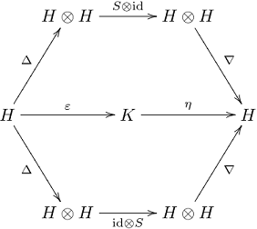
The linear mapping $S\, : \,\mathcal{H}\longrightarrow \mathcal{H}$ is called the antipode of
$$
\mathcal{H}=(\mathcal{H}\, , \,\nabla\, , \,\eta\, , \,\Delta\, , \,\epsilon\, , \,S)
$$
where
$$
S \ast\operatorname{id}=\eta \circ \epsilon = \operatorname{id}\ast S
$$
with a product called folding so that the antipode is the inverse element of the identity mapping. It is not surprising that details become quickly rather technical. I mentioned them because they have diverse applications in physics and string theory. A simple example for a Hopf algebra is a group algebra $\mathcal{H}=\mathbb{F}G$ where $G$ is a group and
$$
\Delta(g)=g\otimes g\; , \;\epsilon(g)=1\; , \;S(g)=g^{-1}.
$$
Another natural example is the universal enveloping algebra $U(\mathfrak{g})$ of a Lie algebra $\mathfrak{g}$ which becomes a Hopf algebra $\mathcal{H}=(U(\mathfrak{g}),\nabla,\eta,\Delta,\epsilon,S)$ by
$$
\Delta(u)=1\otimes u +u\otimes 1\; , \;\epsilon(g)=0\; , \;S(u)=-u.
$$
This makes Hopf algebras relevant for the cohomology theory of Lie groups. There are more example listed on Wikipedia [8].

Boolean Algebras

Boolean algebras are named after the British mathematician and logician George Boole (1815-1864). They are algebras over the field $\mathbb{F}_2=\{0,1\}.$ They have the binary and unary logical operations
$$
\text{AND, OR, NEGATION}
$$
or likewise the binary and unary set operations
$$
\text{UNION, INTERSECTION, COMPLEMENT}.
$$
Boolean algebras are important for combinational circuits and theoretical computer science. E.g. the famous NP-complete satisfiability problem SAT is a statement about expressions in a Boolean algebra. Their formal definition involves about a dozen of rules that we do not need to quote here.

Epilogue

There are many more algebras with specific properties, e.g., a not necessarily associative baric algebra $\mathcal{A}_b$ that has a one-dimensional linear representation, i.e. a homomorphism into the underlying field of scalars. If this mapping is surjective then it is called weight function, which explains the name.

A commutative algebra $\mathcal{G}$ with a basis $\{v_1,\ldots,v_n\}$ is called a genetic algebra if
\begin{align*}
v_i \cdot v_j &=\sum_{k=1}^n \lambda_{ijk} v_k\\
\lambda_{111}&=1\\
\lambda_{1jk}&=0\text{ if }k<j\\
\lambda_{ijk}&=0\text{ if }i,j >1 \text{ and }k \leq \max\{i,j\}
\end{align*}
holds. Every genetic algebra is always a baric algebra [5]. An example of eye colors as a genetic trait can be found in the solution manuals [7] (March 2019, page 422 in the complete file).

I hope I have piqued your interest in the world of algebras. It is a huge world with many still nameless objects. Who knows, maybe one of them will bear your name in the future.

Sources