The LCDM Cosmological Model in Simplified Math (Part 3)
Table of Contents
Part 3: Important Cosmological Horizons and Distances
A question that often comes up is: “how big is the observable universe?”
The question can have more than one answer, depending on the context, so cosmologists have given it a technical name and a precise definition. It is called the ‘particle horizon’, here indicated by Dpar, essentially with the following definition: it is the proper distance that a massless particle, emitted at cosmological time zero, could have bridged until the time it is observed, as judged by the observer.[1] We cannot presently observe anything farther than that, but as time goes on, we will be able to “see farther” (but not necessarily “see more”).
Calculating the Particle Horizon
We have seen the integral for determining the proper distances to a source with stretch S, as is measured by us today (eq. 2.3 of section 2):
3.1 [itex]D_{now} = \int_1^S{\frac{ds}{\sqrt{0.443S^3+1}}}[/itex]
The only difference between the equation for the particle horizon and proper distance today is in the limits of the integral – we have to integrate from today (S=1) all the way to S approaching infinity (as time is extrapolated back to time zero, redshift would extrapolate to infinity).
3.2 [itex]D_{par} = \int_1^{\infty}{\frac{ds}{\sqrt{0.443S^3+1}}} [/itex]
Putting the equation: 1/sqrt(0.443*x^3+1) and values from: ‘1’ to: ‘inf‘ into http://www.numberempire.com/definiteintegralcalculator.php gives the value Dpar = 2.73 lzeit (47.15 Gly). The correct value from LighCone7z is 2.67 lzeit. The reason for the difference is that we necessarily integrate all the way into the radiation-dominated era, for which the simplified equations do not cater. The LightCone7 calculators do cater to radiation energy. However, it is still remarkably close to the correct value for such a simple equation.
In order to get an idea of how the particle horizon have evolved over the history of our universe, we divide by the stretch factor S before the integral and then set the integral limits from S(t) (S at some time ‘t’) to S (approaching) infinity. We then repeat this for the range of time values we want to plot.
3.3 [itex]D_{par}(S) = \frac{1}{S}\int_1^{\infty}{\frac{ds}{\sqrt{0.443S^3+1}}}[/itex]
as shown in the gold curve below:
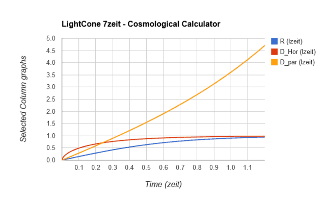
Fig. 3.1 Comparison of Hubble radius, Particle horizon, and Cosmological horizon over time
The Hubble radius (here denoted simply by ‘R’) is just the inverse of the Hubble value (H), e.g. in our units, it has the value ltzeit and numerically it has the same value as the Hubble time (TH). It is how far light could travel in a flat space during one Hubble time. R has a present value of 0.83 lzeit.
The Cosmic Event Horizon
The red curve (DHor) is another form of horizon, the cosmological communications horizon (also called the cosmic event horizon), which is how distant an observer can be and still receive a signal that we transmit today. Or for us to receive (in the future) a signal that the distant observer transmits today. Contrast this to Dpar, which is about information emitted in our past, reaching us today.
As you can see, DHor flattens out at one lzeit and today (t=0.8 zeit), we have a communications horizon of about 0.95 lzeit. It eventually coincides with the Hubble radius.
The equation is essentially the same as for Dpar, but we have to work from today, S=1, to the infinite future, where S = 0 (since ‘a’ goes to infinity and S=1/a).
3.4 [itex]D_{Hor} = \int_0^1{\frac{ds}{\sqrt{0.443S^3+1}}}[/itex]
Presently, we can receive (past) signals from sources that are less than 2.7 lzeit from us, but we can only communicate with receivers that are less than some 0.95 lzeit from us. The reason is that the expansion decelerated in the past, but is presently (and will in the future be) accelerating due to the cosmological constant’s domination.
In order to get an idea of how the cosmic event horizon has evolved over the history of our universe, we divide by the stretch factor S before the integral and then integrate from S at time ‘t’ to S = zero (the ‘infinite future’). We then repeat this for many S (or t) values and plot the curve.
3.5 [itex]D_{Hor}(S) = \frac{1}{S}\int_0^S{\frac{ds}{\sqrt{0.443S^3+1}}}[/itex]
The Hubble Radius Revisited
Finally, we should have a better look at the very important Hubble radius. It is the distance at which the recession rate of an object equals the speed of light. In our natural units, it is simply the inverse of the Hubble constant H at the time. Since H is changing over time, so does the Hubble radius R. I prefer to just use H and R for these parameters, but more formally one should use H(t) and R(t). H(t) is also called the ‘time variable Hubble value’, but note: not the ‘Hubble parameter’, which has a different meaning in cosmology.[2]
Since H (gold) and R (blue) are the inverses of each other, graphically, they look like below, shown together with the (red) lightcone (Dthen) curve of part 2.
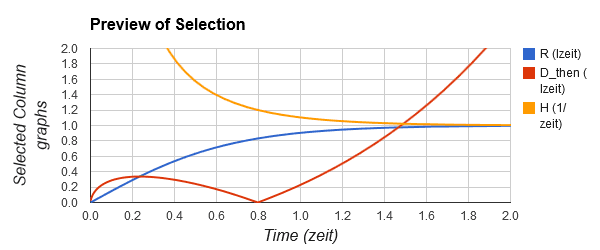
Fig. 3.2 Relationship between Hubble value, Hubble radius, and our Past/Future lightcone.
Since R is a distance in lzeit, the maximum of the red curve happens exactly where it crosses the blue Hubble radius (R) curve, because this is where the proper recession rate equaled the local speed of light. Since R was increasing rather sharply at that time, in-bound photons immediately thereafter found themselves inside our ‘Hubble sphere’ and started to make some headway towards us.[3]
In Section 4, we will conclude this mini-series with a look at the different recession speeds that are of interest in modern cosmology.
End-notes:
[1] Like many other distances, the value of Dpar is model (and model parameter) dependent and cannot be directly measured, but is calculated from other observed parameters, using the model and parameters that fit observational data best.
[2] The Hubble parameter ‘h’ is a dimensionless ratio used in some cosmological equations, expressing the value H0 as a fraction of 100 km/s/Mpc. The present ‘best’ value is h = 0.68, so that (e.g.) the present cosmological time can be expressed as 20.3h Gy. As the value of H0 is refined with better and better measurements, numerical values in some papers do not have to change – the new value for h compensates for that.
[3] Observers at different places in the universe all have their individual Hubble spheres, which may or may not overlap.
Male aerospace engineer
Play music, Read relativity and cosmology


”
Not sure what that would entail—these three pieces seem to form a fairly complete whole—but you might have ideas for a part 4 (although at the moment I can’t think what it might be.”
As I said near the end of part 3, I am thinking that the 3 types of recession rates that we have in the LightCone calculator might be a logical follow-on. Plus perhaps a post-script of some sorts, as you have suggested before (and which you indicated that you are willing to write).
“Maybe there’s something I could write myself that could continue, complement, expand somehow on this base.”
That would be awesome!
“BTW do you plan to ask Greg or someone else on the staff to consolidate the three parts?”
There is a drop down at the top of each article linking the parts together
BTW do you plan to ask Greg or someone else on the staff to consolidate the three parts?
And are you at all tempted to continue and add a part 4 : ^)
Not sure what that would entail—these three pieces seem to form a fairly complete whole—but you might have ideas for a part 4 (although at the moment I can’t think what it might be.)
Maybe there’s something I could write myself that could continue, complement, expand somehow on this base. If you have any ideas for that let me know (if you prefer via PM.)
Jorrie, it’s a fine piece of work! I have to say it was a real delight to see Part 3 when I got up this morning.
It’s nice to see the two main horizons (the cosmic event horizon and the particle horizon) made easily calculable by the reader—and that they make sense as two parts of the same integral. One as the integral from zero to one, and the other as the same integral taken from one to infinity.
Potentially, I think, by giving a newcomer to cosmology a hands-on grasp of how basic features of the universe can be calculated (by anybody!) you make the subject less ad hoc, and above all less frustrating and confusing.