Learn the Fields of Mathematical Quantum Field Theory
The following is one chapter in a series on Mathematical Quantum Field Theory
The previous chapter is 2. Spacetime.
The next chapter is 4. Field variations.
Table of Contents
3. Fields
A field history on a given spacetime ##\Sigma## (a history of spatial field configurations, see remark 3.2 below) is a quantity assigned to each point of spacetime (each event), such that this assignment varies smoothly with spacetime points. For instance, an electromagnetic field history (example 3.6 below) is at each point of spacetime a collection of vectors that encode the direction in which a charged particle passing through that point would feel a force (the “Lorentz force”, see example 3.6 below).
This is readily formalized (def. 3.1 below): If ##F## denotes the smooth manifold of “values” that the given kind of field may take at any spacetime point, then a field history ##\Phi## is modeled as a smooth function from spacetime to this space of values:
$$
\Phi
\;\colon\;
\Sigma
\longrightarrow
F
\,.
$$
It will be useful to unify spacetime and the space of field values (the field fiber) into a single manifold, the Cartesian product
$$
E \;:=\; \Sigma \times F
$$
and to think of this equipped with the projection map onto the first factor as a fiber bundle of spaces of field values over spacetime
$$
\array{
E &:=& \Sigma \times F
\\
{}^{\llap{fb}}\downarrow & \swarrow_{\rlap{pr_1}}
\\
\Sigma
}
\,.
$$
This is then called the field bundle, which specifies the kind of values that the given field species may take at any point of spacetime. Since the space ##F## of field values is the fiber of this fiber bundle (def. 1.9), it is sometimes also called the field fiber. (See also at fiber bundles in physics.)
Given a field bundle ##E \overset{fb}{\to}\Sigma##, then a field history is a section of that bundle (def. 1.7). The discussion of field theory concerns the space of all possible field histories, hence the space of sections of the field bundle (example 3.12 below). This is a very “large” generalized smooth space, called a diffeological space (def. 3.10 below).
Or rather, in the presence of fermion fields such as the Dirac field (example 3.50 below), the Pauli exclusion principle demands that the field bundle is a super-manifold and that the fermionic space of field histories (example 3.51 below) is a super-geometric generalized smooth space: a super smooth set (def. 3.40 below).
This smooth structure on the space of field histories will be crucial when we discuss observables of a field theory below because these are smooth functions on the space of field histories. In particular, it is this smooth structure that allows deriving that linear observables of a free field theory are given by distributions (prop. 7.5) below. Among these are the point evaluation observables (delta distributions) which are traditionally denoted by the same symbol as the field histories themselves.
Hence there are these aspects of the concept of “field” in physics, which are closely related, but crucially different:
aspects of the concept of fields
| aspect | term | type | description | def. |
| field component | ##\phi^a##, ##\phi^a_{,\mu}## | ##J^\infty_\Sigma(E) \to \mathbb{R}## | coordinate function on jet bundle of field bundle | def. 3.1, def. 4.1 |
| field history | ##\Phi##, ##\frac{\partial \Phi}{\partial x^\mu}## | ##\Sigma \to J^\infty_\Sigma(E)## | jet prolongation of section of field bundle | def. 3.1, def. 4.2 |
| field observable | ##\mathbf{\Phi}^a(x)##, ##\partial_{\mu} \mathbf{\Phi}^a(x), ## | ##\Gamma_{\Sigma}(E) \to \mathbb{R}## | derivatives of delta-functional on space of sections | def. 7.1, example 7.2 |
| averaging of field observable | ##\alpha^\ast \mapsto \underset{\Sigma}{\int} \alpha^\ast_a(x) \mathbf{\Phi}^a(x) \, dvol_\Sigma(x)## | ##\Gamma_{\Sigma,cp}(E^\ast) \to Obs(E_{scp},\mathbf{L})## | observable-valued distribution | def. 7.28 |
| algebra of quantum observables | ##\left( Obs(E,\mathbf{L})_{\mu c},\, \star\right)## | ##\mathbb{C}Alg## | non-commutative algebra structure on field observables | def. 14.9, def. 16.1 |
We now discuss these topics:
field bundles
Definition 3.1. (fields and field histories)
Given a spacetime ##\Sigma##, then a type of fields on ##\Sigma## is a smooth fiber bundle (def. 1.9)
$$
\array{E \\ \downarrow^{\rlap{fb}} \\ \Sigma }
$$
called the field bundle,
Given a type of fields on ##\Sigma## this way, then a field history of that type on ##\Sigma## is a term of that type, hence is a smooth section (def. 1.7) of this bundle, namely a smooth function of the form
$$
\Phi \;\colon\; \Sigma \longrightarrow E
$$
such that composed with the projection map it is the identity function, i.e. such that
$$
fb \circ \Phi = id
\phantom{AAAAAAA}
\array{
&& E
\\
& {}^{\llap{\Phi}}\nearrow & \downarrow^{\rlap{fb}}
\\
\Sigma & = & \Sigma
}
\,.
$$
The set of such sections/field histories is to be denoted
| $$ \label{SetOfFieldHistories} \Gamma_\Sigma(E) \;:=\; \left\{ \array{ && E \\ & {}^{\llap{\Phi}}\nearrow & \downarrow^{\rlap{fb}} \\ \Sigma &=& \Sigma } \phantom{fb} \right\} $$ | (18) |
Remark 3.2. (field histories are histories of spatial field configurations)
Given a section ##\Phi \in \Gamma_\Sigma(E)## of the field bundle (def. 3.1) and given a spacelike (def. 2.34) submanifold ##\Sigma_p \hookrightarrow \Sigma## (def. 3.34) of spacetime in codimension 1, then the restriction ##\Phi\vert_{\Sigma_p}## of ##\Phi## to ##\Sigma_p## may be thought of as a field configuration in space. As different spatial slices ##\Sigma_p## are chosen, one obtains such field configurations at different times. It is in this sense that the entirety of a section ##\Phi \in \Gamma_\Sigma(E)## is a history of field configurations, hence a field history (def 3.1).
Remark 3.3. (possible field histories)
After we give the set ##\Gamma_\Sigma(E)## of field histories (18) differential geometric structure, below in example 3.12 and example 3.46, we call it the space of field histories. This should be read as a space of possible field histories; containing all field histories that qualify as being of the type specified by the field bundle ##E##.
After we obtain equations of motion below in def. 5.22, these serve as the “laws of nature” that field histories should obey, and they define the subspace of those field histories that do solve the equations of motion; this will be denoted
$$
\Gamma_\Sigma(E)_{\delta_{EL}\mathbf{L}= 0}
\overset{\phantom{AAA}}{\hookrightarrow}
\Gamma_\Sigma(E)
$$
and called the on-shell space of field histories (40).
For the time being, not to get distracted from the basic idea of quantum field theory, we will focus on the following simple special case of field bundles:
Example 3.4. (trivial vector bundle as a field bundle)
In applications, the field fiber ##F = V## is often a finite-dimensional vector space. In this case, the trivial field bundle with fiber ##F## is of course a trivial vector bundle (def. 1.10).
Choosing any linear basis ##(\phi^a)_{a = 1}^s## of the field fiber, then over Minkowski spacetime (def. 2.17) we have canonical coordinates on the total space of the field bundle
$$
( (x^\mu), ( \phi^a ) )
\,,
$$
where the index ##\mu## ranges from ##0## to ##p##, while the index ##a## ranges from 1 to ##s##.
If this trivial vector bundle is regarded as a field bundle according to def. 3.1, then a field history ##\Phi## is equivalently an ##s##-tuple of real-valued smooth functions ##\Phi^a \colon \Sigma \to \mathbb{R}## on spacetime:
$$
\Phi = ( \Phi^a )_{a = 1}^s
\,.
$$
Example 3.5. (field bundle for real scalar field)
If ##\Sigma## is a spacetime and if the field fiber
$$
F := \mathbb{R}
$$
is simply the real line, then the corresponding trivial field bundle (def. 3.1)
$$
\array{
\Sigma \times \mathbb{R}
\\
{}^{\llap{pr_1}}\downarrow
\\
\Sigma
}
$$
is the trivial real line bundle (a special case of example 3.4) and the corresponding field type (def. 3.1) is called the real scalar field on ##\Sigma##. A configuration of this field is simply a smooth function on ##\Sigma## with values in the real numbers:
| $$ \label{SpaceOfFieldHistoriesOfRealScalarField} \Gamma_\Sigma(\Sigma \times \mathbb{R}) \;\simeq\; C^\infty(\Sigma) \,. $$ | (19) |
Example 3.6. (field bundle for electromagnetic field)
On Minkowski spacetime ##\Sigma## (def. 2.17), let the field bundle (def. 3.1) be given by the cotangent bundle
$$
E := T^\ast \Sigma
\,.
$$
This is a trivial vector bundle (example 3.4) with canonical field coordinates ##(a_\mu)##.
A section of this bundle, hence a field history, is a differential 1-form
$$
A \in \Gamma_\Sigma(T^\ast \Sigma) = \Omega^1(\Sigma)
$$
on spacetime (def. 1.16). Interpreted as a field history of the electromagnetic field on ##\Sigma##, this is often called the vector potential. Then the de Rham differential (def. 1.19) of the vector potential is a differential 2-form
$$
F := d A
$$
known as the Faraday tensor. In the canonical coordinate basis 2-forms this may be expanded as
| $$ \label{TensorFaraday} F = \underset{i = 1}{\overset{p}{\sum}} E_i d x^0 \wedge d x^i + \underset{1 \leq i \lt j \leq p}{\sum} B_{i j} d x^i \wedge d x^j \,. $$ | (20) |
Here ##(E_i)_{i = 1}^p## are called the components of the electric field, while ##(B_{i j})## are called the components of the magnetic field.
Example 3.7. (field bundle for Yang-Mills field over Minkowski spacetime)
Let ##\mathfrak{g}## be a Lie algebra of finite dimension with linear basis ##(t_\alpha)##, in terms of which the Lie bracket is given by
| $$ \label{LieAlgebraStructureConstants} [t_\alpha, t_\beta] \;=\; C^\gamma{}_{\alpha \beta} t_\gamma \,. $$ | (21) |
Over Minkowski spacetime ##\Sigma## (def. 2.17), consider then the field bundle which is the cotangent bundle tensored with the Lie algebra ##\mathfrak{g}##
$$
E := T^\ast \Sigma \otimes \mathfrak{g}
\,.
$$
This is the trivial vector bundle (example 3.4) with induced field coordinates
$$
( a_\mu^\alpha )
\,.
$$
A section of this bundle is a Lie algebra-valued differential 1-form
$$
A \in \Gamma_\Sigma(T^\ast \Sigma \otimes \mathfrak{g}) = \Omega^1(\Sigma, \mathfrak{g})
\,.
$$
with components
$$
A^\ast(a_\mu^\alpha) = A^\alpha_\mu
\,.
$$
This is called a field history for Yang-Mills gauge theory (at least if ##\mathfrak{g}## is a semisimple Lie algebra, see example (42) below).
For ##\mathfrak{g} = \mathbb{R}## is the line Lie algebra, this reduces to the case of the electromagnetic field (example 3.6).
For ##\mathfrak{g} = \mathfrak{su}(3)## this is a field history for the gauge field of the strong nuclear force in quantum chromodynamics.
For readers familiar with the concepts of principal bundles and connections on a bundle we include the following example 3.8 which generalizes the Yang-Mills field over Minkowski spacetime from example 3.7
to the situation over general spacetimes.
Example 3.8. (general Yang-Mills field in fixed topological sector)
Let ##\Sigma## be any spacetime manifold and let ##G## be a compact Lie group with Lie algebra denoted ##\mathfrak{g}##. Let ##P \overset{is}{\to} \Sigma## be a ##G##-principal bundle and ##\nabla_0## a chosen connection on it, to be called the background ##G##-Yang-Mills field.
Then the field bundle (def. 3.1) for ##G##-Yang-Mills theory in the topological sector ##P## is the tensor product of vector bundles
$$
E := \left(P \times^{ad}_G \mathfrak{g}\right) \otimes_\Sigma \left( T^\ast \Sigma \right)
$$
of the adjoint bundle of ##P## and the cotangent bundle of ##\Sigma##.
With the choice of ##\nabla_0##, every (other) connection ##\nabla## on ##P## uniquely decomposes as
$$
\nabla = \nabla_0 + A
\,,
$$
where
$$
A \in \Gamma_\Sigma(E)
$$
is a section of the above field bundle, hence a Yang-Mills field.
The electromagnetic field (def. 3.6) and the Yang-Mills field (def. 3.7, def. 3.8) with differential 1-forms as field histories are the basic examples of gauge fields (we consider this in more detail below in Gauge symmetries). There are also higher gauge fields with differential n-forms as field histories:
Example 3.9. (field bundle for B-field)
On Minkowski spacetime ##\Sigma## (def. 2.17), let the field bundle (def. 3.1) be given by the skew-symmetrized tensor product of vector bundles of the cotangent bundle with itself
$$
E := \wedge^2_\Sigma T^\ast \Sigma
\,.
$$
This is a trivial vector bundle (example 3.4) with canonical field coordinates ##(b_{\mu \nu})## subject to
$$
b_{\mu \nu} \;=\; – b_{\nu \mu}
\,.
$$
A section of this bundle, hence a field history, is a differential 2-form (def. 1.18)
$$
B \in \Gamma_\Sigma(\wedge^2_\Sigma T^\ast \Sigma) = \Omega^2(\Sigma)
$$
on spacetime.
space of field histories
Given any field bundle, we will eventually need to regard the set of all field histories ##\Gamma_\Sigma(E)## as a “smooth set” itself, a smooth space of sections, to which constructions of differential geometry apply (such as for the discussion of observables and states below ). Notably, we need to be talking about differential forms on ##\Gamma_\Sigma(E)##.
However, a space of sections ##\Gamma_\Sigma(E)## does not, in general, carry the structure of a smooth manifold; and it carries the correct smooth structure of an infinite-dimensional manifold only if ##\Sigma## is a compact space (see at the manifold structure of mapping spaces). Even if it does carry infinite-dimensional manifold structure, inspection shows that this is more structure than actually needed for the discussion of field theory. Namely, it turns out below that all we need to know is what counts as a smooth family of sections/field histories, hence which functions of sets
$$
\Phi_{(-)} \;\colon\; \mathbb{R}^n \longrightarrow \Gamma_\Sigma(E)
$$
from any Cartesian space ##\mathbb{R}^n## (def. 1.1) into ##\Gamma_\Sigma(E)## count as smooth functions, subject to some basic consistency condition on this choice.
This structure on ##\Gamma_\Sigma(E)## is called the structure of a diffeological space:
Definition 3.10. (diffeological space)
A diffeological space ##X## is
- a set ##X_s \in ## Set;
- for each ##n \in \mathbb{N}## a choice of subset$$
X(\mathbb{R}^n) \subset Hom_{Set}(\mathbb{R}^n_s, X_s) = \left\{ \mathbb{R}^n_s \to X_s \right\}
$$of the set of functions from the underlying set ##\mathbb{R}^n_s## of ##\mathbb{R}^n## to ##X_s##, to be called the smooth functions or plots from ##\mathbb{R}^n## to ##X##; - for each smooth function ##f \;\colon\; \mathbb{R}^{n_1} \longrightarrow \mathbb{R}^{n_2}## between Cartesian spaces (def. 1.1) a choice of function$$
f^\ast \;\colon\; X(\mathbb{R}^{n_2}) \longrightarrow X(\mathbb{R}^{n_1})
$$to be thought of as the precomposition operation$$
\left(
\mathbb{R}^{n_2} \overset{\Phi}{\longrightarrow} X
\right)
\;\overset{f^\ast}{\mapsto}\;
\left(
\mathbb{R}^{n_1} \overset{f}{\to} \mathbb{R}^{n_2} \overset{\Phi}{\to} X
\right)
$$
such that
- (constant functions are smooth)$$
X(\mathbb{R}^0) = X_s
\,,
$$ - (functionality)
- If ##id_{\mathbb{R}^n} \;\colon\; \mathbb{R}^n \to \mathbb{R}^n## is the identity function on ##\mathbb{R}^n##, then ##\left(id_{\mathbb{R}^n}\right)^\ast \;\colon\; X(\mathbb{R}^n) \to X(\mathbb{R}^n)## is the identity function on the set of plots ##X(\mathbb{R}^n)##;
- If ##\mathbb{R}^{n_1} \overset{f}{\to} \mathbb{R}^{n_2} \overset{g}{\to} \mathbb{R}^{n_3}## are two composable smooth functions between Cartesian spaces (def. 1.1), then pullback of plots along them consecutively equals the pullback along the composition:$$
f^\ast \circ g^\ast
=
(g \circ f)^\ast
$$i.e.$$
\array{
&& X(\mathbb{R}^{n_2})
\\
& {}^{\llap{f^\ast}}\swarrow && \nwarrow^{\rlap{g^\ast}}
\\
X(\mathbb{R}^{n_1})
&& \underset{ (g \circ f)^\ast }{\longleftarrow} &&
X(\mathbb{R}^{n_3})
}
$$
- (gluing)If ##\{ U_i \overset{f_i}{\to} \mathbb{R}^n\}_{i \in I}## is a differentiably good open cover of a Cartesian space (def. 1.5) then the function which restricts ##\mathbb{R}^n##-plots of ##X## to a set of ##U_i##-plots$$
X(\mathbb{R}^n)
\overset{( (f_i)^\ast )_{i \in I} }{\hookrightarrow}
\underset{i \in I}{\prod} X(U_i)
$$is a bijection onto the set of those tuples ##(\Phi_i \in X(U_i))_{i \in I}## of plots, which are “matching families” in that they agree on intersections:$$
\phi_i\vert_{U_i \cap U_j} = \phi_j \vert_{U_i \cap U_j}
\phantom{AAAAAA}
\array{
&& U_i \cap U_j
\\
& \swarrow && \searrow
\\
U_i && && U_j
\\
& {}_{\rlap{\Phi_i}}\searrow && \swarrow_{\rlap{\Phi_j}}
\\
&& X
}
$$
Finally, given ##X_1## and ##X_2## two diffeological spaces, then a smooth function between them
$$
f \;\colon\; X_1 \longrightarrow X_2
$$
is
- a function of the underlying sets$$
f_s \;\colon\; (X_1)_s \longrightarrow (X_2)_s
$$
such that
- for ##\Phi \in X(\mathbb{R}^n)## a plot of ##X_1##, then the composition ##f_s \circ \Phi_s## is a plot ##f_\ast(\Phi)## of ##X_2##:$$
\array{
&& \mathbb{R}^n
\\
& {}^{\llap{\Phi}}\swarrow && \searrow^{\rlap{f_\ast(\Phi)}}
\\
X_1 && \underset{f}{\longrightarrow} && X_2
}
\,.
$$
(Stated more abstractly, this says simply that diffeological spaces are the concrete sheaves on the site of Cartesian spaces from def. 1.5.)
For more background on diffeological spaces see also the geometry of physics — smooth sets.
Example 3.11. (Cartesian spaces are diffeological spaces)
Let ##X## be a Cartesian space (def. 1.1) Then it becomes a diffeological space (def. 3.10) by declaring its plots ##\Phi \in X(\mathbb{R}^n)## to the ordinary smooth functions ##\Phi \colon \mathbb{R}^n \to X##.
Under this identification, a function ##f \;\colon\; (X_1)_s \to (X_2)_s## between the underlying sets of two Cartesian spaces is a smooth function in the ordinary sense precisely if it is a smooth function in the sense of diffeological spaces.
Stated more abstractly, this statement is an example of the Yoneda embedding over a subcanonical site.
More generally, the same construction makes every smooth manifold a smooth set.
Example 3.12. (diffeological space of field histories)
Let ##E \overset{fb}{\to} \Sigma## be a smooth field bundle (def. 3.1). Then the set ##\Gamma_\Sigma(E)## of field histories/sections (def. 3.1) becomes a diffeological space (def. 3.10)
| $$ \label{SpaceOfFieldHistories} \Gamma_\Sigma(E) \in DiffeologicalSpaces $$ | (22) |
by declaring that a smooth family ##\Phi_{(-)}## of field histories, parameterized over any Cartesian space ##U## is a smooth function out of the Cartesian product manifold of ##\Sigma## with ##U##
$$
\array{
U \times \Sigma &\overset{\Phi_{(-)}(-)}{\longrightarrow}& E
\\
(u,x) &\mapsto& \Phi_u(x)
}
$$
such that for each ##u \in U## we have ##p \circ \Phi_{u}(-) = id_\Sigma##, i.e.
$$
\array{
&& E
\\
& {}^{\llap{\Phi_{(-)}(-)}}\nearrow & \downarrow^{\rlap{fb}}
\\
U \times \Sigma &\underset{pr_2}{\longrightarrow}& \Sigma
}
\,.
$$
The following example 3.13 is included only for readers who wonder how infinite-dimensional manifolds fit in. Since we will never actually use infinite-dimensional manifold structure, this example is may be ignored.
Example 3.13. (Fréchet manifolds are diffeological spaces)
Consider the particular type of infinite-dimensional manifolds called Fréchet manifolds. Since ordinary smooth manifolds ##U## is an example, for ##X## a Fréchet manifold there is a concept of smooth functions ##U \to X##. Hence we may give ##X## the structure of a diffeological space (def. 3.10) by declaring the plots over ##U## to be these smooth functions ##U \to X##, with the evident post-composition action.
It turns out that then that for ##X## and ##Y## two Fréchet manifolds, there is a natural bijection between the smooth functions ##X \to Y## between them regarded as Fréchet manifolds and [regarded as diffeological spaces. Hence it does not matter which of the two perspectives we take (unless of course, a diffeological space more general than a Fréchet manifold enters the picture, at which point the second definition generalizes, whereas the first does not).
Stated more abstractly, this means that Fréchet manifolds form a full subcategory of that of diffeological spaces (this prop.):
$$
FrechetManifolds \hookrightarrow DiffeologicalSpaces
\,.
$$
If ##\Sigma## is a compact smooth manifold and ##E \simeq \Sigma \times F \to \Sigma## is a trivial fiber bundle with fiber ##F## a smooth manifold, then the set of sections ##\Gamma_\Sigma(E)## carries a standard structure of a Fréchet manifold (see at manifold structure of mapping spaces). Under the above inclusion of Fréchet manifolds into diffeological spaces, this smooth structure agrees with that from example 3.12 (see this prop.)
Once the step from smooth manifolds to diffeological spaces (def. 3.10) is made, characterizing the smooth structure of the space entirely by how we may probe it by mapping smooth Cartesian spaces into it, it becomes clear that the underlying set ##X_s## of a diffeological space ##X## is not actually crucial to support the concept: The space is already entirely defined structurally by the system of smooth plots it has, and the underlying set ##X_s## is recovered from these as the set of plots from the point ##\mathbb{R}^0##.
This is crucial for field theory: the spaces of field histories of fermionic fields (def. 3.45 below) such as the Dirac field (example 3.51 below) do not have underlying sets of points the way diffeological spaces have. Informally, the reason is that a point is a bosonic object, while and the nature of fermionic fields is the opposite of bosonic.
But we may just as well drop the mentioning of the underlying set ##X_s## in the definition of generalized smooth spaces. By simply stripping this requirement off of def. 3.10 we obtain the following more general and more useful definition (still “bosonic”, though, the supergeometric version is def. 3.40 below):
Definition 3.14. (smooth set)
A smooth set ##X## is
- for each ##n \in \mathbb{N}## a choice of set$$
X(\mathbb{R}^n) \in Set
$$to be called the set of smooth functions or plots from ##\mathbb{R}^n## to ##X##; - for each smooth function ##f \;\colon\; \mathbb{R}^{n_1} \longrightarrow \mathbb{R}^{n_2}## between Cartesian spaces a choice of function$$
f^\ast \;\colon\; X(\mathbb{R}^{n_2}) \longrightarrow X(\mathbb{R}^{n_1})
$$to be thought of as the precomposition operation$$
\left(
\mathbb{R}^{n_2} \overset{\Phi}{\longrightarrow} X
\right)
\;\overset{f^\ast}{\mapsto}\;
\left(
\mathbb{R}^{n_1} \overset{f}{\to} \mathbb{R}^{n_2} \overset{\Phi}{\to} X
\right)
$$
such that
- (functionality)
- If ##id_{\mathbb{R}^n} \;\colon\; \mathbb{R}^n \to \mathbb{R}^n## is the identity function on ##\mathbb{R}^n##, then ##\left(id_{\mathbb{R}^n}\right)^\ast \;\colon\; X(\mathbb{R}^n) \to X(\mathbb{R}^n)## is the identity function on the set of plots ##X(\mathbb{R}^n)##.
- If ##\mathbb{R}^{n_1} \overset{f}{\to} \mathbb{R}^{n_2} \overset{g}{\to} \mathbb{R}^{n_3}## are two composable smooth functions between Cartesian spaces, then consecutive pullback of plots along them equals the pullback along the composition:$$
f^\ast \circ g^\ast
=
(g \circ f)^\ast
$$i.e.$$
\array{
&& X(\mathbb{R}^{n_2})
\\
& {}^{\llap{f^\ast}}\swarrow && \nwarrow^{\rlap{g^\ast}}
\\
X(\mathbb{R}^{n_1})
&& \underset{ (g \circ f)^\ast }{\longleftarrow} &&
X(\mathbb{R}^{n_3})
}
$$
- (gluing)If ##\{ U_i \overset{f_i}{\to} \mathbb{R}^n\}_{i \in I}## is a differentiably good open cover of a Cartesian space (def. 1.5) then the function which restricts ##\mathbb{R}^n##-plots of ##X## to a set of ##U_i##-plots$$
X(\mathbb{R}^n)
\overset{( (f_i)^\ast )_{i \in I} }{\hookrightarrow}
\underset{i \in I}{\prod} X(U_i)
$$is a bijection onto the set of those tuples ##(\Phi_i \in X(U_i))_{i \in I}## of plots, which are “matching families” in that they agree on intersections:$$
\phi_i\vert_{U_i \cap U_j} = \phi_j \vert_{U_i \cap U_j}
\phantom{AAAA}
\text{i.e.}
\phantom{AAAA}
\array{
&& U_i \cap U_j
\\
& \swarrow && \searrow
\\
U_i && && U_j
\\
& {}_{\rlap{\Phi_i}}\searrow && \swarrow_{\rlap{\Phi_j}}
\\
&& X
}
$$
Finally, given ##X_1## and ##X_2## two smooth sets, then a smooth function between them
$$
f \;\colon\; X_1 \longrightarrow X_2
$$
is
- for each ##n \in \mathbb{N}## a function$$
f_\ast(\mathbb{R}^n)
\;\colon\;
X_1(\mathbb{R}^n) \longrightarrow X_2(\mathbb{R}^n)
$$
such that
- for each smooth function ##g \colon \mathbb{R}^{n_1} \to \mathbb{R}^{n_2}## between Cartesian spaces we have$$
g^\ast_2 \circ f_\ast(\mathbb{R}^{n_2})
=
f_\ast(\mathbb{R}^{n_1}) \circ g^\ast_1
\phantom{AAAAA}
\text{i.e.}
\phantom{AAAAA}
\text{i.e.}
\phantom{AAAAA}
\array{
X_1(\mathbb{R}^{n_2})
&\overset{f_\ast(\mathbb{R}^{n_2})}{\longrightarrow}&
X_2(\mathbb{R}^{n_2})
\\
\llap{g_1^\ast}\downarrow && \downarrow\rlap{g^\ast_2}
\\
X_1(\mathbb{R}^{n_1})
&\underset{f_\ast(\mathbb{R}^{n_1})}{\longrightarrow}&
X_2(\mathbb{R}^{n_1})
}
$$
Stated more abstractly, this simply says that smooth sets are the _sheaves on the site of Cartesian spaces from def. 1.5.
Basing differential geometry on smooth sets is an instance of the general approach to geometry called functorial geometry or topos theory. For more background on this see at geometry of physics — smooth sets.
First we verify that the concept of smooth sets is a consistent generalization:
Example 3.15. (diffeological spaces are smooth sets)
Every diffeological space ##X## (def. 3.10) is a smooth set (def. 3.14) simply by forgetting its underlying set of points and remembering only its sets of plot.
In particular therefore each Cartesian space ##\mathbb{R}^n## is canonically a smooth set by example 3.11.
Moreover, given any two diffeological spaces, then the morphisms ##f \colon X \to Y## between them, regarded as diffeological spaces, are the same as the morphisms as smooth sets.
Stated more abstractly, this means that we have full subcategory inclusions
$$
CartesianSpaces
\overset{\phantom{AAA}}{\hookrightarrow}
DiffeologicalSpaces
\overset{\phantom{AAA}}{\hookrightarrow}
SmoothSets
\,.
$$
Recall, for the next proposition 3.16, that in the definition 3.14 of a smooth set ##X## the sets ##X(\mathbb{R}^n)## are abstract sets which are to be thought of as would-be smooth functions “##\mathbb{R}^n \to X##”. Inside def. 3.14 this only makes sense in quotation marks, since inside that definition the smooth set ##X## is only being defined, so that inside that definition there is not yet an actual concept of smooth functions of the form “##\mathbb{R}^n \to X##”.
But now that the definition of smooth sets and of morphisms between them has been stated, and seeing that Cartesian space ##\mathbb{R}^n## are examples of smooth sets, by example 3.15, there is now an actual concept of smooth functions ##\mathbb{R}^n \to X##, namely as smooth sets. For the concept of smooth sets to be consistent, it ought to be true that this a posteriori concept of smooth functions from Cartesian spaces to smooth sets coincides with the a priori concept, hence that we “may remove the quotation marks” in the above. The following proposition says that this is indeed the case:
Proposition 3.16. (plots of a smooth set really are the smooth functions into the smooth set)
Let ##X## be a smooth set (def. 3.14). For ##n \in \mathbb{R}##, there is a natural function
$$
Hom_{SmoothSet}(\mathbb{R}^n , X) \overset{\phantom{AA}\simeq\phantom{AA}}{\longrightarrow} X(\mathbb{R}^n)
$$
from the set of homomorphisms of smooth sets from ##\mathbb{R}^n## (regarded as a smooth set via example 3.15) to ##X##, to the set of plots of ##X## over ##\mathbb{R}^n##, given by evaluating on the identity plot ##id_{\mathbb{R}^n}##.
This function is a bijection.
This says that the plots of ##X##, which initially bootstrap ##X## into being as declaring the would-be smooth functions into ##X##, end up being the actual smooth functions into ##X##.
Proof. This elementary but profound fact is called the Yoneda lemma, here in its incarnation over the site of Cartesian spaces (def. 1.1).
A key class of examples of smooth sets (def. 3.14) that are not diffeological spaces (def. 3.10) are universal smooth moduli spaces of differential forms:
Example 3.17. (universal smooth moduli spaces of differential forms)
For ##k \in \mathbb{N}## there is a smooth set (def. 3.14)
$$
\mathbf{\Omega}^k \;\in\; SmoothSet
$$
defined as follows:
- for ##n \in \mathbb{N}## the set of plots from ##\mathbb{R}^n## to ##\mathbf{\Omega}^k## is the set of smooth differential k-forms on ##\mathbb{R}^n## (def. 1.18)$$
\mathbf{\Omega}^k(\mathbb{R}^n) \;:=\; \Omega^k(\mathbb{R}^n)
$$ - for ##f \colon \mathbb{R}^{n_1} \to \mathbb{R}^{n_2}## a smooth function (def. 1.1) the operation of fullback of plots along ##f## is just the pullback of differential forms ##f^\ast## from prop. 1.21
$$
\array{
\mathbb{R}^{n_1} && \Omega^k(\mathbb{R}^{n_1})
\\
\downarrow^{\rlap{f}} && \uparrow^{\rlap{f^\ast}}
\\
\mathbb{R}^{n_2} && \Omega^k(\mathbb{R}^{n_2})
}
$$
That this is functorial is just the standard fact (7) from prop. 1.21.
For ##k = 1## the smooth set ##\mathbf{\Omega}^0## actually is a diffeological space, in fact under the identification of example 3.15 this is just the real line:
$$
\mathbf{\Omega}^0 \simeq \mathbb{R}^1
\,.
$$
But for ##k \geq 1## we have that the set of plots on ##\mathbb{R}^0 = \ast## is a singleton
$$
\mathbf{\Omega}^{k \geq 1}(\mathbb{R}^0) \simeq \{0\}
$$
consisting just of the zero differential form. The only diffeological space with this property is ##\mathbb{R}^0 = \ast## itself. But ##\mathbf{\Omega}^{k \geq 1}## is far from being that trivial: even though its would-be underlying set is a single point, for all ##n \geq k## it admits an infinite set of plots. Therefore the smooth sets ##\mathbf{\Omega}^k## for ##k \geq## are not diffeological spaces.
That the smooth set ##\mathbf{\Omega}^k## indeed deserves to be addressed as the universal moduli space of differential k-forms follows from prop. 3.16: The universal moduli space of ##k##-forms ought to carry a universal differential ##k##-forms ##\omega_{univ} \in \Omega^k(\mathbf{\Omega}^k)## such that every differential ##k##-form ##\omega## on any ##\mathbb{R}^n## arises as the pullback of differential forms of this universal one along some modulating morphism ##f_\omega \colon X \to \mathbf{\Omega}^k##:
$$
\array{
\{\omega\} &\overset{(f_\omega)^\ast}{\longleftarrow}& \{\omega_{univ}\}
\\
\\
X &\underset{f_\omega}{\longrightarrow}& \mathbf{\Omega}^k
}
$$
But with prop. 3.16 this is precisely what the definition of the plots of ##\mathbf{\Omega}^k## says.
Similarly, all the usual operations on differential form now have their universal archetype on the universal moduli spaces of differential forms
In particular, for ##k \in \mathbb{N}## there is a canonical morphism of smooth sets of the form
$$
\mathbf{\Omega}^k \overset{\mathbf{d}}{\longrightarrow} \mathbf{\Omega}^{k+1}
$$
defined over ##\mathbb{R}^n## by the ordinary de Rham differential (def. 1.19)
| $$ \label{deRhamDifferentialUniversal} \Omega^k(\mathbb{R}^n) \overset{d}{\longrightarrow} \Omega^{k+1}(\mathbb{R}^n) \,. $$ | (23) |
That this satisfies the compatibility with pre-composition of plots
$$
\array{
\mathbb{R}^{n_1} && \Omega^k(\mathbb{R}^{n_1}) &\overset{d}{\longrightarrow}& \Omega^{k+1}(\mathbb{R}^{n_1})
\\
{}^{\llap{f}}\downarrow && \uparrow^{\rlap{f^\ast}} && \uparrow^{\rlap{f^\ast}}
\\
\mathbb{R}^{n_2} && \Omega^k(\mathbb{R}^{n_2}) &\underset{d}{\longrightarrow}& \Omega^k( \mathbb{R}^{n_2} )
}
$$
is just the compatibility of pullback of differential forms with the de Rham differential of from prop. 1.21.
The upshot is that we now have a good definition of differential forms on any diffeological space and more generally on any smooth set:
Definition 3.18. (differential forms on smooth sets)
Let ##X## be a diffeological space (def. 3.10) or more generally a smooth set (def. 3.14) then a differential k-form ##\omega## on ##X## is equivalently a morphism of smooth sets
$$
X \longrightarrow \mathbf{\Omega}^k
$$
from ##X## to the universal smooth moduli space of differential froms from example 3.17.
Concretely, by unwinding the definitions of ##\mathbf{\Omega}^k## and of morphisms of smooth sets, this means that such a differential form is:
- for each ##n \in \mathbb{N}## and each plot ##\mathbb{R}^n \overset{\Phi}{\to} X## an ordinary differential form$$
\Phi^\ast(\omega) \in \Omega^\bullet(\mathbb{R}^n)
$$
such that
- for each smooth function ##f \;\colon\; \mathbb{R}^{n_1} \to \mathbb{R}^{n_2}## between Cartesian spaces the ordinary pullback of differential forms along ##f## is compatible with these choices, in that for every plot ##\mathbb{R}^{n_2} \overset{\Phi}{\to} X## we have$$
f^\ast\left(\Phi^\ast(\omega)\right)
=
( f^\ast \Phi )^\ast(\omega)
$$i.e.$$
\array{
\mathbb{R}^{n_1} && \overset{f}{\longrightarrow} && \mathbb{R}^{n_2}
\\
& {}_{\llap{f^\ast \Phi}}\searrow && \swarrow_{\rlap{\Phi}}
\\
&& X
}
\phantom{AAAA}
\array{
\Omega^\bullet( \mathbb{R}^{n_1} ) && \overset{f^\ast}{\longleftarrow} && \Omega^\bullet(\mathbb{R}^{n_2})
\\
& {}_{\llap{(f^\ast \Phi)^\ast}}\nwarrow && \nearrow_{\rlap{\Phi^\ast}}
\\
&& \Omega^\bullet(X)
}
\,.
$$
We write ##\Omega^\bullet(X)## for the set of differential forms on the smooth set ##X## defined this way.
Moreover, given a differential k-form
$$
X \overset{\omega}{\longrightarrow} \mathbf{\Omega}^k
$$
on a smooth set ##X## this way, then its de Rham differential ##d \omega \in \Omega^{k+1}(X)## is given by the composite of morphisms of smooth sets with the universal de Rham differential from (23):
| $$ \label{FormsOnSmoothSetDeRhamDifferential} d \omega \;\colon\; X \overset{\omega}{\longrightarrow} \mathbf{\Omega}^k \overset{d}{\longrightarrow} \mathbf{\Omega}^{k+1} \,. $$ | (24) |
Explicitly this means simply that for ##\Phi \colon U \to X## a plot, then
$$
\Phi^\ast (d\omega)
\;=\;
d\left( \Phi^\ast \omega\right)
\;\in\;
\Omega^{k+1}(U)
\,.
$$
The usual operations on ordinary differential forms directly generalize plot-wise to differential forms on diffeological spaces and more generally on smooth sets:
Definition 3.19. (exterior differential and exterior product on smooth sets)
Let ##X## be a diffeological space (def. 3.10) or more generally a smooth set (def. 3.14). Then
- For ##\omega \in \Omega^n(X)## a differential form on ##X## (def. 3.18) its exterior differential$$
d \omega \in \Omega^{n+1}(X)
$$is defined on any plot ##\mathbb{R}^n \overset{\Phi}{\to} X## as the ordinary exterior differential of the pullback of ##\omega## along that plot:$$
\Phi^\ast(d \omega) := d \Phi^\ast(\omega)
\,.
$$ - For ##\omega_1 \in \Omega^{n_1}## and ##\omega_2 \in \Omega^{n_2}(X)## two differential forms on ##X## (def. 3.18) then their exterior product$$
\omega_1 \wedge \omega_2 \;\in\; \Omega^{n_1 + n_2}(X)
$$is the differential form defined on any plot ##\mathbb{R}^n \overset{\Phi}{\to} X## as the ordinary exterior product of the pullback of th differential forms ##\omega_1## and ##\omega_2## to this plot:$$
\Phi^\ast(\omega_1 \wedge \omega_2)
\;:=\;
\Phi^\ast(\omega_1) \wedge \Phi^\ast(\omega_2)
\,.
$$
Infinitesimal geometry
It is crucial in field theory that we consider field histories not only over all of the spacetime but also restricted to submanifolds of spacetime. Or rather, what is actually of interest are the restrictions of the field histories to the infinitesimal neighborhoods (example 3.30 below) of these submanifolds. This appears notably in the construction of phase spaces below. Moreover, fermion fields such as the Dirac field (example 3.50 below) take values in graded infinitesimal spaces, called super spaces (discussed below). Therefore “infinitesimal geometry”, sometimes called formal geometry (as in “formal scheme”) or synthetic differential geometry or synthetic differential supergeometry, is a central aspect of field theory.
In order to mathematically grasp what infinitesimal neighborhoods are, we appeal to the first magic algebraic property of differential geometry from prop. 1.15, which says that we may recognize smooth manifolds ##X## dually in terms of their commutative algebras ##C^\infty(X)## of smooth functions on them
$$
C^\infty(-) \;\colon\; SmoothManifolds \overset{\phantom{AAA}}{\hookrightarrow} (\mathbb{R} Algebras)^{op}
\,.
$$
But since there are of course more algebras ##A \in \mathbb{R}Algebras## than arise this way from smooth manifolds, we may turn this around and try to regard any algebra ##A## as defining a would-be space, which would have ##A## as its algebra of functions.
For example, an infinitesimally thickened point should be a space that is “so small” that every smooth function ##f## on it which vanishes at the origin takes values so tiny that some finite power of them is not just even tinier, but actually vanishes:
Definition 3.20. (infinitesimally thickened Cartesian space)
An infinitesimally thickened point
$$
\mathbb{D} := Spec(A)
$$
is represented by a commutative algebra ##A \in \mathbb{R}Alg## which as real vector space is a direct sum
$$
A \simeq_{\mathbb{R}} \langle 1 \rangle \oplus V
$$
of the 1-dimensional space ##\langle 1 \rangle = \mathbb{R}## of multiples of 1 with a finite dimensional vector space ##V## that is a nilpotent ideal in that for each element ##a \in V## there exists a natural number ##n \in \mathbb{N}## such that
$$
a^{n+1} = 0
\,.
$$
More generally, an infinitesimally thickened Cartesian space
$$
\mathbb{R}^n \times \mathbb{D} \;:=\; \mathbb{R}^n \times Spec(A)
$$
is represented by a commutative algebra
$$
C^\infty(\mathbb{R}^n) \otimes A \;\in\; \mathbb{R} Alg
$$
which is the tensor product of algebras of the algebra of smooth functions ##C^\infty(\mathbb{R}^n)## on an actual Cartesian space of some dimension ##n## (example 1.3), with an algebra of functions ##A \simeq_{\mathbb{R}} \langle 1\rangle \oplus V## of an infinitesimally thickened point, as above.
We say that a smooth function between two infinitesimally thickened Cartesian spaces
$$
\mathbb{R}^{n_1} \times Spec(A_1) \overset{f}{\longrightarrow} \mathbb{R}^{n_2} \times Spec(A_2)
$$
is by definition dually an ##\mathbb{R}##-algebra homomorphism of the form
$$
C^\infty(\mathbb{R}^{n_1}) \otimes A_1
\overset{f^\ast}{\longleftarrow}
C^\infty(\mathbb{R}^{n_2}) \otimes A_2
\,.
$$
Example 3.21. (infinitesimal neighborhoods in the real line )
Consider the quotient algebra of the formal power series algebra ##\mathbb{R}[ [\epsilon] ]## in a single parameter ##\epsilon## by the ideal generated by ##\epsilon^2##:
$$
(\mathbb{R}[ [\epsilon] ])/(\epsilon^2)
\;\simeq_{\mathbb{R}}\;
\mathbb{R} \oplus \epsilon \mathbb{R}
\,.
$$
(This is sometimes called the algebra of dual numbers, for no good reason.) The underlying real vector space of this algebra is, as shown, the direct sum of the multiples of 1 with the multiples of ##\epsilon##. A general element in this algebra is of the form
$$
a + b \epsilon \in (\mathbb{R}[\epsilon])/(\epsilon^2)
$$
where ##a,b \in \mathbb{R}## are real numbers. The product in this algebra is given by “multiplying out” as usual, and discarding all terms proportional to ##\epsilon^2##:
$$
\left(
a_1 + b_1 \epsilon
\right)
\cdot
\left(
a_2 + b_2 \epsilon
\right)
\;=\;
a_1 a_2 + ( a_1 b_2 + b_1 a_2 ) \epsilon
\,.
$$
We may think of an element ##a + b \epsilon## as the truncation to the first order of a Taylor series at the origin of a smooth function on the real line
$$
f \;\colon\; \mathbb{R} \to \mathbb{R}
$$
where ##a = f(0)## is the value of the function at the origin, and where ##b = \frac{\partial f}{\partial x}(0)## is its first derivative at the origin.
Therefore this algebra behaves like the algebra of smooth function on an infinitesimal neighborhood ##\mathbb{D}^1## of ##0 \in \mathbb{R}## which is so tiny that its elements ##\epsilon \in \mathbb{D}^1 \hookrightarrow \mathbb{R}## become, upon squaring them, not just tinier, but actually zero:
$$
\epsilon^2 = 0
\,.
$$
This intuitive picture is now made precise by the concept of infinitesimally thickened points def. 3.20, if we simply set
$$
\mathbb{D}^1
\;:=\;
Spec\left(
\mathbb{R}[ [\epsilon] ]/(\epsilon^2)
\right)
$$
and observe that there is the inclusion of infinitesimally thickened Cartesian spaces
$$
\mathbb{D}^1 \overset{\phantom{AA}i\phantom{AA} }{\hookrightarrow} \mathbb{R}^1
$$
which is dually given by the algebra homomorphism
$$
\array{
\mathbb{R} \oplus \epsilon \mathbb{R}
&\overset{i^\ast}{\longleftarrow}&
C^\infty(\mathbb{R}^1)
\\
f(0) + \frac{\partial f}{\partial x}(0) &\longleftarrow& \{f\}
}
$$
which sends a smooth function to its value ##f(0)## at zero plus ##\epsilon## times its derivative at zero. Observe that this is indeed a homomorphism of algebras due to the product law of differentiation>, which says that
$$
\begin{aligned}
i^\ast(f \cdot g)
& =
(f \cdot g)(0) + \frac{\partial f \cdot g}{\partial x}(0) \epsilon
\\
& =
f(0) \cdot g(0)
+
\left(
\frac{\partial f}{\partial x}(0) \cdot g(0) + f(0) \cdot \frac{\partial g}{\partial x}(0)
\right) \epsilon
\\
& =
\left(
f(0) + \frac{\partial f}{\partial x}(0) \epsilon
\right)
\cdot
\left(
g(0) + \frac{\partial g}{\partial x}(0) \epsilon
\right)
\end{aligned}
$$
Hence we see that restricting a smooth function to the infinitesimal neighborhood of a point is equivalent to restricting attention to its [[Taylor series|] to the given order at that point:
$$
\array{
\mathbb{D}^1 &\overset{i}{\hookrightarrow}& \mathbb{R}^1
\\
& {}_{\llap{(\epsilon \mapsto f(0) + \frac{\partial f}{\partial x}(0) \epsilon) }}\searrow & \downarrow_{\rlap{f}}
\\
&& \mathbb{R}^1
}
$$
Similarly for each ##k \in \mathbb{N}## the algebra
$$
(\mathbb{R}[ [ \epsilon ] ])/(\epsilon^{k+1})
$$
may be thought of as the algebra of Taylor series at the origin of ##\mathbb{R}## of smooth functions ##\mathbb{R} \to \mathbb{R}##, where all terms of order higher than ##k## are discarded. The corresponding infinitesimally thickened point is often denoted
$$
\mathbb{D}^1(k) \;:=\; Spec\left( \left(\mathbb{R}[ [\epsilon] ]\right)/(\epsilon^{k+1}) \right)
\,.
$$
This is now the subobject of the real line
$$
\mathbb{D}^1(k) \overset{\phantom{AAA}}{\hookrightarrow} \mathbb{R}^1
$$
on those elements ##\epsilon## such that ##\epsilon^{k+1} = 0##.
(Kock 81, Kock 10)
The following example 3.22 shows that infinitesimal thickening is invisible for ordinary spaces when mapping out of these. In contrast example 3.23 further below shows that the morphisms into an ordinary space out of an infinitesimal space are interesting: these are tangent vectors and their higher-order infinitesimal analogs.
Example 3.22. (infinitesimal line ##\mathbb{D}^1## has a unique global point)
For ##\mathbb{R}^n## any ordinary Cartesian space (def. 1.1) and ##D^1(k) \hookrightarrow \mathbb{R}^1## the order-##k## infinitesimal neighborhood of the origin in the real line from example 3.21, there is exactly only one possible morphism of infinitesimally thickened Cartesian spaces from ##\mathbb{R}^n## to ##\mathbb{D}^1(k)##:
$$
\array{
\mathbb{R}^n && \overset{\exists !}{\longrightarrow} &6 \mathbb{D}^1(k)
\\
& {}_{\llap{\exists !}}\searrow && \nearrow_{\rlap{\exists !}}
\\
&& \mathbb{R}^0 = \ast
}
\,.
$$
Proof. By definition, such a morphism is dually an algebra homomorphism
$$
C^\infty(\mathbb{R}^n)
\overset{f^\ast}{\longleftarrow}
\left(
\mathbb{R}[ [\epsilon] ])/(\epsilon^{k+1}
\right)
\simeq_{\mathbb{R}}
\mathbb{R} \oplus \mathcal{O}(\epsilon)
$$
from the higher-order “algebra of dual numbers” to the algebra of smooth functions (example 1.3).
Now, this being an ##\mathbb{R}##-algebra homomorphism, its action on the multiples ##c \in \mathbb{R}## of the identity is fixed:
$$
f^\ast(1) = 1
\,.
$$
All the remaining elements are proportional to ##\epsilon##, and hence are nilpotent. However, by the homomorphism property of an algebra homomorphism it follows that it must send nilpotent elements ##\epsilon## to nilpotent elements ##f(\epsilon)##, because
$$
\begin{aligned}
\left(f^\ast(\epsilon)\right)^{k+1}
& = f^\ast\left( \epsilon^{k+1}\right)
\\
& = f^\ast(0)
\\ & = 0
\end{aligned}
$$
But the only nilpotent element in ##C^\infty(\mathbb{R}^n)## is the zero elements, and hence it follows that
$$
f^\ast(\epsilon) = 0
\,.
$$
Thus ##f^\ast## as above is uniquely fixed.
Example 3.23. (synthetic tangent vector fields)
Let ##\mathbb{R}^n## be a Cartesian space (def. 1.1), regarded as an infinitesimally thickened Cartesian space (def. 3.20) and consider ##\mathbb{D}^1 := Spec( (\mathbb{R}[ [\epsilon] ])/(\epsilon^2) )## the first order infinitesimal line from example 3.21.
Then homomorphisms of infinitesimally thickened Cartesian spaces of the form
$$
\array{
\mathbb{R}^n \times \mathbb{D}^1
&& \overset{\tilde v}{\longrightarrow} &&
\mathbb{R}^n
\\
& {}_{\llap{pr_1}}\searrow && \swarrow_{\rlap{id}}
\\
&& \mathbb{R}^n
}
$$
hence smoothly ##X##-parameterized collections of morphisms
$$
\tilde v_x \;\colon\; \mathbb{D}^1 \longrightarrow \mathbb{R}^n
$$
which send the unique base point ##\Re(\mathbb{D}^1) = \ast## (example 3.22) to ##x \in \mathbb{R}^n##, are in natural bijection with tangent vector fields ##v \in \Gamma_{\mathbb{R}^n}(T \mathbb{R}^n)## (example 1.12).
Proof. By definition, the morphisms in question are dually ##\mathbb{R}##-algebra homomorphisms of the form
$$
(C^\infty(\mathbb{R}^n) \oplus \epsilon C^\infty(\mathbb{R}^n))
\longleftarrow
C^\infty(\mathbb{R}^n)
$$
which are the identity modulo ##\epsilon##. Such a morphism has to take any function ##f \in C^\infty(\mathbb{R}^n)## to
$$
f + (\partial f) \epsilon
$$
for some smooth function ##(\partial f) \in C^\infty(\mathbb{R}^n)##. The condition that this assignment makes an algebra homomorphism is equivalent to the statement that for all ##f_1,f_2 \in C^\infty(\mathbb{R}^n)## we have
$$
(f_1 f_2 + (\partial (f_1 f_2))\epsilon )
\;=\;
(f_1 + (\partial f_1) \epsilon)
\cdot
(f_2 + (\partial f_2) \epsilon)
\,.
$$
Multiplying this out and using that ##\epsilon^2 = 0##, this is equivalent to
$$
\partial(f_1 f_2) = (\partial f_1) f_2 + f_1 (\partial f_2)
\,.
$$
This in turn means equivalently that ##\partial\colon C^\infty(\mathbb{R}^n)\to C^\infty(\mathbb{R}^n)## is a derivation.
With this the statement follows with the third magic algebraic property of smooth functions (prop. 1.15): derivations of smooth functions are vector fields.
We need to consider infinitesimally thickened spaces more general than the thickenings of just Cartesian spaces in def. 3.20. But just as Cartesian spaces (def. 1.1) serve as the local test geometries to induce the general concept of diffeological spaces and smooth sets (def. 3.14), so using infinitesimally thickened Cartesian spaces as test geometries immediately induces the corresponding generalization of smooth sets with infinitesimals:
Definition 3.24. (formal smooth set)
A formal smooth set ##X## is
- for each infinitesimally thickened Cartesian space ##\mathbb{R}^n \times Spec(A)## (def. 3.20) a set$$
X(\mathbb{R}^n \times Spec(A)) \in Set
$$to be called the set of smooth functions or plots from ##\mathbb{R}^n \times Spec(A)## to ##X##; - for each smooth function ##f \;\colon\; \mathbb{R}^{n_1} \times Spec(A_1) \longrightarrow \mathbb{R}^{n_2} \times Spec(A_2)## between infinitesimally thickened Cartesian spaces a choice of function$$
f^\ast \;\colon\; X(\mathbb{R}^{n_2} \times Spec(A_2)) \longrightarrow X(\mathbb{R}^{n_1} \times Spec(A_1))
$$to be thought of as the precomposition operation$$
\left(
\mathbb{R}^{n_2} \overset{\Phi}{\longrightarrow} X
\right)
\;\overset{f^\ast}{\mapsto}\;
\left(
\mathbb{R}^{n_1}\times Spec(A_1) \overset{f}{\to} \mathbb{R}^{n_2} \times Spec(A_2) \overset{\Phi}{\to} X
\right)
$$
such that
- (functionality)
- If ##id_{\mathbb{R}^n \times Spec(A)} \;\colon\; \mathbb{R}^n \times Spec(A) \to \mathbb{R}^n \times Spec(A)## is the identity function on ##\mathbb{R}^n \times Spec(A)##, then ##\left(id_{\mathbb{R}^n \times Spec(A)}\right)^\ast \;\colon\; X(\mathbb{R}^n \times Spec(A)) \to X(\mathbb{R}^n \times Spec(A))## is the identity function on the set of plots ##X(\mathbb{R}^n \times Spec(A))##;
- If ##\mathbb{R}^{n_1}\times Spec(A_1) \overset{f}{\to} \mathbb{R}^{n_2} \times Spec(A_2) \overset{g}{\to} \mathbb{R}^{n_3} \times Spec(A_3)## are two composable smooth functions between infinitesimally thickened Cartesian spaces, then pullback of plots along them consecutively equals the pullback along the composition:$$
f^\ast \circ g^\ast = (g \circ f)^\ast
$$i.e.$$
\array{
&& X(\mathbb{R}^{n_2} \times Spec(A_2))
\\
& {}^{\llap{f^\ast}}\swarrow && \nwarrow^{\rlap{g^\ast}}
\\
X(\mathbb{R}^{n_1} \times Spec(A_1))
&& \underset{ (g \circ f)^\ast }{\longleftarrow} &&
X(\mathbb{R}^{n_3} \times Spec(A_3))
}
$$
- (gluing)If ##\{ U_i \times Spec(A) \overset{f_i \times id_{Spec(A)}}{\to} \mathbb{R}^n \times Spec(A)\}_{i \in I}## is such that $$\{ U_i \overset{f_i }{\to} \mathbb{R}^n \}_{i \in I}$$ in a differentiably good open cover (def. 1.5) then the function which restricts ##\mathbb{R}^n \times Spec(A)##-plots of ##X## to a set of ##U_i \times Spec(A)##-plots$$
X(\mathbb{R}^n \times Spec(A))
\overset{( (f_i)^\ast )_{i \in I} }{\hookrightarrow}
\underset{i \in I}{\prod} X(U_i \times Spec(A))
$$is a bijection onto the set of those tuples ##(\Phi_i \in X(U_i))_{i \in I}## of plots, which are “matching families” in that they agree on intersections:$$
\phi_i\vert_{((U_i \cap U_j) \times Spec(A)} = \phi_j \vert_{(U_i \cap U_j)\times Spec(A)}
$$i.e.$$
\array{
&& (U_i \cap U_j) \times Spec(A)
\\
& \swarrow && \searrow
\\
U_i\times Spec(A) && && U_j \times Spec(A)
\\
& {}_{\rlap{\Phi_i}}\searrow && \swarrow_{\rlap{\Phi_j}}
\\
&& X
}
$$
Finally, given ##X_1## and ##X_2## two formal smooth sets, then a smooth function between them
$$
f \;\colon\; X_1 \longrightarrow X_2
$$
is
- for each infinitesimally thickened Cartesian space ##\mathbb{R}^n \times Spec(A)## (def. 3.20) a function$$
f_\ast(\mathbb{R}^n \times Spec(A))
\;\colon\;
X_1(\mathbb{R}^n \times Spec(A)) \longrightarrow X_2(\mathbb{R}^n \times Spec(A))
$$
such that
- for each smooth function ##g \colon \mathbb{R}^{n_1} \times Spec(A_1) \to \mathbb{R}^{n_2} \times Spec(A_2)## between infinitesimally thickened Cartesian spaces we have$$
g^\ast_2 \circ f_\ast(\mathbb{R}^{n_2} \times Spec(A_2))
=
f_\ast(\mathbb{R}^{n_1} \times Spec(A_1)) \circ g^\ast_1
$$i.e.$$
\array{
X_1(\mathbb{R}^{n_2} \times Spec(A_2))
&\overset{f_\ast(\mathbb{R}^{n_2}\times Spec(A_2) )}{\longrightarrow}&
X_2(\mathbb{R}^{n_2} \times Spec(A_2))
\\
\llap{g_1^\ast}\downarrow && \downarrow\rlap{g^\ast_2}
\\
X_1(\mathbb{R}^{n_1} \times Spec(A_1))
&\underset{f_\ast(\mathbb{R}^{n_1})}{\longrightarrow}&
X_2(\mathbb{R}^{n_1} \times Spec(A_1))
}
$$
(Dubuc 79)
Basing infinitesimal geometry on formal smooth sets is an instance of the general approach to geometry called functorial geometry or topos theory. For more background on this see at geometry of physics — manifolds and orbifolds.
We have the evident generalization of example 3.11 to smooth geometry with infinitesimals:
Example 3.25. (infinitesimally thickened Cartesian spaces are formal smooth sets)
For ##X## an infinitesimally thickened Cartesian space (def. 3.20), it becomes a formal smooth set according to def. 3.24
by taking its plots out of some ##\mathbb{R}^n \times \mathbb{D}## to be the homomorphism of infinitesimally thickened Cartesian spaces:
$$
X(\mathbb{R}^n \times \mathbb{D})
\;:=\;
Hom_{FormalCartSp}( \mathbb{R}^n \times \mathbb{D}, X )
\,.
$$
(Stated more abstractly, this is an instance of the Yoneda embedding over a subcanonical site.)
Example 3.26. (smooth sets are formal smooth sets)
Let ##X## be a smooth set (def. 3.14). Then ##X## becomes a formal smooth set (def. 3.24) by declaring the set of plots ##X(\mathbb{R}^n \times \mathbb{D})## over an infinitesimally thickened Cartesian space (def. 3.20) to be equivalence classes of pairs
$$
\mathbb{R}^n \times \mathbb{D} \longrightarrow \mathbb{R}^{k}
\,,
\phantom{AA}
\mathbb{R}^k \longrightarrow X
$$
of a morphism of infinitesimally thickened Cartesian spaces and of a plot of ##X##, as shown, subject to the equivalence relation which identifies two such pairs if there exists a smooth function ##f \colon \mathbb{R}^k \to \mathbb{R}^{k’}## such that
$$
\array{
&& \mathbb{R}^n \times \mathbb{D}
\\
& \swarrow && \searrow
\\
\mathbb{R}^k && \overset{f}{\longrightarrow} && \mathbb{R}^{k’}
\\
\mathbb{R}^k && \underset{f}{\longrightarrow} && \mathbb{R}^{k’}
\\
& \searrow && \swarrow
\\
&& X
}
$$
Stated more abstractly this says that ##X## as a formal smooth set is the left Kan extension (see this example) of ##X## as a smooth set along the functor that includes Cartesian spaces (def. 1.1) into infinitesimally thickened Cartesian spaces (def. 3.20).
Definition 3.27. (reduction and infinitesimal shape)
For ##\mathbb{R}^n \times \mathbb{D}## an infinitesimally thickened Cartesian space (def. 3.20) we say that the underlying ordinary Cartesian space ##\mathbb{R}^n## (def. 1.1) is its reduction
$$
\Re\left(
\mathbb{R}^n \times \mathbb{D}
\right)
\;:=\;
\mathbb{R}^n
\,.
$$
There is the canonical inclusion morphism
$$
\Re\left(
\mathbb{R}^n \times \mathbb{D}
\right)
=
\mathbb{R}^n
\overset{\phantom{AAAA}}{\hookrightarrow}
\mathbb{R}^n \times \mathbb{D}
$$
which dually corresponds to the homomorphism of commutative algebras
$$
C^\infty(\mathbb{R}^n)
\longleftarrow
C^\infty(\mathbb{R}^n)
\otimes_{\mathbb{R}}
A
$$
which is the identity on all smooth functions ##f \in C^\infty(\mathbb{R}^n)## and is zero on all elements ##a \in V \subset A## in the nilpotent ideal of ##A## (as in example 3.22).
Given any formal smooth set ##X##, we say that its infinitesimal shape or de Rham shape (also: de Rham stack) is the formal smooth set ##\Im X## (def. 3.24) defined to have as plots the reductions of the plots of ##X##, according to the above:
$$
(\Im X)( U ) \;:=\: X(\Re(U))
\,.
$$
There is a canonical morphism of formal smooth set
$$
\eta_X
\;\colon\;
X
\longrightarrow
\Im X
$$
which takes a plot
$$
U = \mathbb{R}^n \times \mathbb{D} \overset{f}{\longrightarrow} X
$$
to the composition
$$
\mathbb{R}^n \hookrightarrow \mathbb{R}^n \times \mathbb{D} \overset{f}{\hookrightarrow} X
$$
regarded as a plot of ##\Im X##.
Example 3.28. (mapping space out of an infinitesimally thickened Cartesian space)
Let ##X## be an infinitesimally thickened Cartesian space (def. 3.20) and let ##Y## be a formal smooth set (def. 3.24). Then the mapping space
$$
[X,Y] \;\in\; FormalSmoothSet
$$
of smooth functions from ##X## to ##Y## is the formal smooth set whose ##U##-plots are the morphisms of formal smooth sets from the Cartesian product of infinitesimally thickened Cartesian spaces ##U \times X## to ##Y##, hence the ##U \times X##-plots of ##Y##:
$$
[X,Y](U) \;:=\; Y(U \times X)
\,.
$$
Example 3.29. (synthetic tangent bundle)
Let ##X := \mathbb{R}^n## be a Cartesian space (def. 1.1) regarded as an infinitesimally thickened Cartesian space (3.20) and thus regarded as a formal smooth set (def. 3.24) by example 3.25. Consider the infinitesimal line
$$
\mathbb{D}^1
\hookrightarrow
\mathbb{R}^1
$$
from example 3.21. Then the mapping space ##[\mathbb{D}^1, X]## (example 3.28) is the total space of the tangent bundle ##T X## (example 1.12). Moreover, under restriction along the reduction ##\ast \longrightarrow \mathbb{D}^1##, this is the full tangent bundle projection, in that there is a natural isomorphism of formal smooth sets of the form
$$
\array{
T X &\simeq& [\mathbb{D}^1, X]
\\
{}^{\llap{tb}}\downarrow && \downarrow^{\rlap{ [ \ast \to \mathbb{D}^1, X ] }}
\\
X &\simeq& [\ast, X]
}
$$
In particular, this implies immediately that smooth sections (def. 1.7) of the tangent bundle
$$
\array{
&& [\mathbb{D}^1, X] & \simeq T X
\\
& {}^{\llap{v}}\nearrow & \downarrow
\\
X &=& X
}
$$
are equivalently morphisms of the form
$$
\array{
&& X
\\
& {}^{\llap{\tilde v}}\nearrow & \downarrow^{\rlap{id}}
\\
X \times \mathbb{D}^1 &\underset{pr_1}{\longrightarrow}& X
}
$$
which we had already identified with tangent vector fields (def. 1.12) in example 3.23.
Proof. This follows by an analogous argument as in example 3.23, using the Hadamard lemma.
While in infinitesimally thickened Cartesian spaces (def. 3.20) only infinitesimals to any finite order may exist, in formal smooth sets (def. 3.24) we may find infinitesimals to any arbitrary finite order:
Example 3.30. (infinitesimal neighborhood)
Let ##X## be a formal smooth sets (def. 3.24) ##Y \hookrightarrow X## a sub-formal smooth set. Then the infinitesimal neighborhood to arbitrary infinitesimal order of ##Y## in ##X## is the formal smooth set ##N_X Y## whose plots are those plots of ##X##
$$
\mathbb{R}^n \times Spec(A) \overset{f}{\longrightarrow} X
$$
such that their reduction (def. 3.27)
$$
\mathbb{R}^n \hookrightarrow \mathbb{R}^n \times Spec(A) \overset{f}{\longrightarrow} X
$$
factors through a plot of ##Y##.
This allows grasping the restriction of field histories to the infinitesimal neighborhood of a submanifold of spacetime, which will be crucial for the discussion of phase spaces below.
Definition 3.31. (field histories on infinitesimal neighborhood of submanifold of spacetime)
Let ##E \overset{fb}{\to} \Sigma## be a field bundle (def. 3.1) and let ##S \hookrightarrow \Sigma## be a submanifold of spacetime.
We write ##N_\Sigma(S) \hookrightarrow \Sigma## for its infinitesimal neighbourhood in ##\Sigma## (def. 3.30).
Then the set of field histories restricted to ##S##, to be denoted
| $$ \label{SpaceOfFieldHistoriesInHigherCodimension} \Gamma_{S}(E) := \Gamma_{N_\Sigma(S)}( E\vert_{N_\Sigma S} ) \in \mathbf{H} $$ | (25) |
is the set of section of ##E## restricted to the infinitesimal neighbourhood ##N_\Sigma(S)## (example 3.30).
We close the discussion of infinitesimal differential geometry by explaining how we may recover the concept of smooth manifolds inside the more general formal smooth sets (def./prop. 3.34 below). The key point is that the presence of infinitesimals in the theory allows an intrinsic definition of local diffeomorphisms/formally étale morphism (def. 3.32 and example 3.33 below). It is noteworthy that the only role this concept plays in the development of field theory below is that smooth manifolds admit triangulations by smooth singular simplices (def. 1.23) so that the concept of fiber integration of differential forms is well defined over manifolds.
Definition 3.32. (local diffeomorphism of formal smooth sets)
Let ##X,Y## be formal smooth sets (def. 3.24). Then a morphism between them is called a local diffeomorphism or formally étale morphism, denoted
$$
f \;\colon\; X \overset{et}{\longrightarrow} Y
\,,
$$
if ##f## if for each infinitesimally thickened Cartesian space (def. 3.20) ##\mathbb{R}^n \times \mathbb{D}## we have a natural identification between the ##\mathbb{R}^n \times \mathbb{D}##-plots of ##X## with those ##\mathbb{R}^n n\times \mathbb{D}##-plots of ##Y## whose reduction (def. 3.27) comes from an ##\mathbb{R}^n##-plot of ##X##, hence if we have a natural fiber product of sets of plots
$$
X(\mathbb{R}^n \times \mathbb{D})
\;\simeq\;
Y(\mathbb{R}^n \times \mathbb{D})
\underset{Y(\mathbb{R}^n)}{\times^f}
X(\mathbb{R}^n)
$$
i. e.
$$
\array{
&& X(\mathbb{R}^n \times \mathbb{D})
\\
& \swarrow && \searrow
\\
Y(\mathbb{R}^n \times \mathbb{D}) && \text{(pb)} && X(\mathbb{R}^n)
\\
& \searrow && \swarrow
\\
&& Y(\mathbb{R}^n )
}
$$
for all infinitesimally thickened Cartesian spaces ##\mathbb{R}^n \times \mathbb{D}##.
Stated more abstractly, this means that the naturality square of the unit of the infinitesimal shape ##\Im## (def. 3.27) is a pullback square
$$
\array{
X &\overset{\eta_X}{\longrightarrow}& \Im X
\\
{}^{\llap{f}}\downarrow &\text{(pb)}& \downarrow^{\rlap{\Im f}}
\\
Y &\underset{\eta_Y}{\longrightarrow}& \Im Y
}
$$
(Khavkine-Schreiber 17, def. 3.1)
Example 3.33. (local diffeomorphism between Cartesian spaces from the general definition)
For ##X,Y \in CartSp## two ordinary Cartesian spaces (def. 1.1), regarded as formal smooth sets by example 3.25 then a morphism ##f \colon X \to Y## between them is a local diffeomorphism in the general sense of def. 3.32
precisely if it is so in the ordinary sense of def. 1.4.
(Khavkine-Schreiber 17, prop. 3.2)
Definition/Proposition 3.34. (smooth manifolds)
A smooth manifold ##X## of dimension ##n \in \mathbb{N}## is
- a diffeological space (def. 3.10)
such that
- there exists an indexed set ##\{ \mathbb{R}^n \overset{\phi_i}{\to} X\}_{i \in I}## of morphisms of formal smooth sets (def. 3.24) from Cartesian spaces ##\mathbb{R}^n## (def. 1.1) (regarded as formal smooth sets via example 3.11, example 3.15 and example 3.26) into ##X##, (regarded as a formal smooth set via example 3.15 and example 3.26) such that
- every point ##x \in X_s## is in the image of at least one of the ##\phi_i##;
- every ##\phi_i## is a local diffeomorphism according to def. 3.32;
- the final topology induced by the set of plots of ##X## makes ##X_s## a paracompact Hausdorff space.
(Khavkine-Schreiber 17, example 3.4)
For more on smooth manifolds from the perspective of formal smooth sets see at the geometry of physics — manifolds and orbifolds.
fermion fields and supergeometry
Field theories of interest crucially involve fermionic fields (def. 3.45 below), such as the Dirac field (example 3.50 below), which are subject to the “Pauli exclusion principle”, a key reason for the stability of matter. Mathematically this principle means that these fields have field bundles whose field fiber is not an ordinary manifold, but an odd-graded supermanifold (more on this in remark 5.21 and remark 5.29 below).
This “supergeometry” is an immediate generalization of the infinitesimal geometry above, where now the infinitesimal elements in the algebra of functions may be equipped with a grading: one speaks of superalgebra.
The “super”-terminology for something as down-to-earth as the mathematical principle behind the stability of matter may seem unfortunate. For better or worse, this terminology has become standard since the middle of the 20th century. But the concept that today is called supercommutative superalgebra was in fact first considered by Grassmann in 1844 who got it right (“Ausdehnungslehre”) but apparently was too far ahead of his time and remained unappreciated.
Beware that considering supergeometry does not necessarily involve considering “supersymmetry”. Supergeometry is the geometry of fermion fields (def. 3.45 below), and that all matter fields in the observable universe are fermionic has been experimentally established since the Stern-Gerlach experiment in 1922. Supersymmetry, on the other hand, is a hypothetical extension of spacetime-symmetry within the context of supergeometry. Here we do not discuss supersymmetry; for details see instead at the geometry of physics — supersymmetry.
Definition 3.35. (supercommutative superalgebra)
A real ##\mathbb{Z}/2##-graded algebra or superalgebra is an associative algebra ##A## over the real numbers together with a direct sum decomposition of its underlying real vector space
$$
A \simeq_{\mathbb{R}} A_{even} \oplus A_{odd}
\,,
$$
such that the product in the algebra respects the multiplication in the cyclic group of order 2 ##\mathbb{Z}/2 = \{even, odd\}##:
$$
\left.
\array{
A_{even} \cdot A_{even}
\\
A_{odd} \cdot A_{odd}
}
\right\}
\subset A_{even}
\phantom{AAAA}
\left.
\array{
A_{odd} \cdot A_{even}
\\
A_{even} \cdot A_{odd}
}
\right\}
\subset A_{odd}
\,.
$$
This is called a supercommutative superalgebra if for all elements ##a_1, a_2 \in A## which are of homogeneous degree ##{\vert a_i \vert} \in \mathbb{Z}/2 = \{even, odd\}## in that
$$
a_i \in A_{{\vert a_i\vert}} \subset A
$$
we have
$$
a_1 \cdot a_2 = (-1)^{{\vert a_1 \vert \vert a_2 \vert}} a_2 \cdot a_1
\,.
$$
A homomorphism of superalgebras
$$
f \;\colon\; A \longrightarrow A’
$$
is a homomorphism of associative algebras over the real numbers such that the ##\mathbb{Z}/2##-grading is respected in that
$$
f(A_{even}) \subset A’_{even}
\phantom{AAAAA}
f(A_{odd}) \subset A’_{odd}
\,.
$$
For more details on superalgebra see at the geometry of physics — superalgebra.
Example 3.36. (basic examples of supercommutative superalgebras)
Basic examples of supercommutative superalgebras (def. 3.35) include the following:
- Every commutative algebra ##A## becomes a supercommutative superalgebra by declaring it to be all in even degree: ##A = A_{even}##.
- For ##V## a finite dimensional real vector space, then the Grassmann algebra ##A := \wedge^\bullet_{\mathbb{R}} V^\ast## is a supercommutative superalgebra with ##A_{even} := \wedge^{even} V^\ast## and ##A_{odd} := \wedge^{odd} V^\ast##.More explicitly, if ##V = \mathbb{R}^s## is a Cartesian space with canonical dual coordinates ##(\theta^i)_{i = 1}^s## then the Grassmann algebra ##\wedge^\bullet (\mathbb{R}^s)^\ast## is the real algebra which is generated from the ##\theta^i## regarded in odd degree and hence subject to the relation$$
\theta^i \cdot \theta^j = – \theta^j \cdot \theta^i
\,.
$$In particular this implies that all the ##\theta^i## are infinitesimal (def. 3.20):$$
\theta^i \cdot \theta^i = 0
\,.
$$ - For ##A_1## and ##A_2## two supercommutative superalgebras, there is their tensor product supercommutative superalgebra ##A_1 \otimes_{\mathbb{R}} A_2##. For example for ##X## a smooth manifold with the ordinary algebra of smooth functions ##C^\infty(X)## regarded as a supercommutative superalgebra by the first example above, the tensor product with a Grassmann algebra (second example above) is supercommutative superalgebta$$
C^\infty(X) \otimes_{\mathbb{R}} \wedge^\bullet((\mathbb{R}^s)\ast)
$$whose elements may uniquely be expanded in the form$$
f + f_i \theta^i + f_{i j} \theta^i \theta^j + f_{i j k} \theta^i \theta^j \theta^k + \cdots + f_{i_1 \cdots i_s} \theta^{i_1} \cdots \theta^{i_s}
\,,
$$where the ##f_{i_1 \cdots i_k} \in C^\infty(X)## are smooth functions on ##X## which are skew-symmetric in their indices.
The following is the direct super-algebraic analog of the definition of infinitesimally thickened Cartesian spaces (def. 3.20):
Definition 3.37. (super Cartesian space)
A superpoint ##Spec(A)## is represented by a super-commutative superalgebra ##A## (def. 3.35) which as a ##\mathbb{Z}/2##-graded vector space (super vector space) is a direct sum
$$
A \simeq_{\mathbb{R}} \langle 1 \rangle \oplus V
$$
of the 1-dimensional even vector space ##\langle 1 \rangle = \mathbb{R}## of multiples of 1, with a finite dimensional super vector space ##V## that is a nilpotent ideal in ##A## in that for each element ##a \in V## there exists a natural number ##n \in \mathbb{N}## such that
$$
a^{n+1} = 0
\,.
$$
More generally, a super Cartesian space ##\mathbb{R}^n \times Spec(A)## is represented by a super-commutative algebra ##C^\infty(\mathbb{R}^n) \otimes A \in \mathbb{R} Alg## which is the tensor product of algebras of the algebra of smooth functions ##C^\infty(\mathbb{R}^n)## on an actual Cartesian space of some dimension ##n##, with an algebra of functions ##A \simeq_{\mathbb{R}} \langle 1\rangle \oplus V## of a superpoint (example 3.36).
Specifically, for ##s \in \mathbb{N}##, there is the superpoint
| $$ \label{StandardSuperpoints} \mathbb{R}^{0 \vert s} \;:=\; Spec\left( \wedge^\bullet (\mathbb{R}^s)^\ast \right) $$ | (26) |
whose algebra of functions is by definition the Grassmann algebra on ##s## generators ##(\theta^i)_{i = 1}^s## in odd degree (example 3.36).
We write
$$
\begin{aligned}
\mathbb{R}^{b\vert s}
& :=
\mathbb{R}^b \times \mathbb{R}^{0 \vert s}
\\
& =
\mathbb{R}^b \times Spec( \wedge^\bullet(\mathbb{R}^s)^\ast )
\\
& =
Spec\left( C^\infty(\mathbb{R}^b) \otimes_{\mathbb{R}} \wedge^\bullet (\mathbb{R}^s)^\ast \right)
\end{aligned}
$$
for the corresponding super Cartesian spaces whose algebra of functions is as in example 3.36.
We say that a smooth function between two super Cartesian spaces
$$
\mathbb{R}^{n_1} \times Spec(A_1) \overset{f}{\longrightarrow} \mathbb{R}^{n_2} \times Spec(A_2)
$$
is by definition dually a homomorphism of supercommutative superalgebras (def. 3.35) of the form
$$
C^\infty(\mathbb{R}^{n_1}) \otimes A_1
\overset{f^\ast}{\longleftarrow}
C^\infty(\mathbb{R}^{n_2}) \otimes A_2
\,.
$$
Example 3.38. (superpoint induced by a finite-dimensional vector space)
Let ##V## be a finite-dimensional real vector space. With ##V^\ast## denoting its 3.37).
We denote this superpoint by
$$
V_{odd} \simeq \mathbb{R}^{0 \vert dim(V)}
\,.
$$
All the differential geometry over Cartesian space that we discussed above generalizes immediately to super Cartesian spaces (def. 3.37) if we strictly adhere to the super sign rule which says that whenever two odd-graded elements swap places, a minus sign is picked up. In particular, we have the following generalization of the de Rham complex on Cartesian spaces discussed above.
Definition 3.39. (super differential forms on super Cartesian spaces)
For ##\mathbb{R}^{b\vert s}## a super Cartesian space (def. 3.37), hence the formal dual of the supercommutative superalgebra of the form
$$
C^\infty(\mathbb{R}^{b\vert s})
\;=\;
C^\infty(\mathbb{R}^b) \otimes_{\mathbb{R}} \wedge^\bullet \mathbb{R}^s
$$
with canonical even-graded coordinate functions ##(x^i)_{i = 1^b}## and odd-graded coordinate functions ##(\theta^j)_{j = 1}^s##.
Then the de Rham complex of super differential forms on ##\mathbb{R}^{b\vert s}## is, in super-generalization of def. 1.18, the ##\mathbb{Z} \times (\mathbb{Z}/2)##-graded commutative algebra
$$
\Omega^\bullet(\mathbb{R}^{b|s})
\;:=\;
C^\infty(\mathbb{R}^{b|s})
\otimes_{\mathbb{R}}
\wedge^\bullet \langle
d x^1, \cdots, d x^b,
\;
d \theta^1, \cdots, d\theta^s
\rangle
$$
which is generated over ##C^\infty(\mathbb{R}^{b\vert s})## from new generators
$$
\underset{
\text{deg} = (1,even)
}{\underbrace{ d x^i }}
\phantom{AAAAA}
\underset{
\text{deg} = (1,odd)
}{
\underbrace{
d \theta^j
}
}
$$
whose differential is defined in degree-0 by
$$
d f
\;:=\;
\frac{\partial f}{\partial x^i} d x^i
+
\frac{\partial f}{\partial \theta^j} d \theta^j
$$
and extended from there as a bigraded derivation of bi-degree ##(1,even)##, in super-generalization of def. 1.19.
Accordingly, the operation of contraction with tangent vector fields (def. 1.20) has bi-degree ##(-1,\sigma)## if the tangent vector has super-degree ##\sigma##:
| generator | bi-degree |
| ##\phantom{AA} x^a## | (0,even) |
| ##\phantom{AA} \theta^\alpha## | (0,odd) |
| ##\phantom{AA} dx^a## | (1,even) |
| ##\phantom{AA} d\theta^\alpha## | (1,odd) |
| derivation | bi-degree |
| ##\phantom{AA} d## | (1,even) |
| ##\phantom{AA}\iota_{\partial x^a}## | (-1, even) |
| ##\phantom{AA}\iota_{\partial \theta^\alpha}## | (-1,odd) |
This means that if ##\alpha \in \Omega^\bullet(\mathbb{R}^{b\vert s})## is in bidegree ##(n_\alpha, \sigma_\alpha)##, and ##\beta \in \Omega^\bullet(\mathbb{R}^{b \vert \sigma})## is in bidegree ##(n_\beta, \sigma_\beta)##, then
$$
\alpha \wedge \beta
\;
=
\;
(- 1)^{n_\alpha n_\beta + \sigma_\alpha \sigma_\beta}
\;
\beta \wedge \alpha
\,.
$$
Hence there are two contributions to the sign picked up when exchanging two super-differential forms in the wedge product:
- there is a “cohomological sign” which for commuting an ##n_1##-forms past an ##n_2##-form is ##(-1)^{n_1 n_2}##;
- in addition there is a “super-grading” sign which for commuting a ##\sigma_1##-graded coordinate function past a ##\sigma_2##-graded coordinate function (possibly under the de Rham differential) is ##(-1)^{\sigma_1 \sigma_2}##.
For example:
$$
x^{a_1} (dx^{a_2}) \;=\; + (dx^{a_2}) x^{a_1}
$$
$$
\theta^\alpha (dx^a) \;=\; + (dx^a) \theta^\alpha
$$
$$
\theta^{\alpha_1} (d\theta^{\alpha_2})
\;=\;
– (d\theta^{\alpha_2}) \theta^{\alpha_1}
$$
$$
dx^{a_1}
\wedge
d x^{a_2}
\;=\;
–
d x^{a_2}
\wedge
d x^{a_1}
$$
$$
dx^a
\wedge
d \theta^{\alpha}
\;=\;
–
d\theta^{\alpha}
\wedge
d x^a
$$
$$
d\theta^{\alpha_1}
\wedge
d \theta^{\alpha_2}
\;=\;
+
d\theta^{\alpha_2}
\wedge
d \theta^{\alpha_1}
$$
(e.g. Castellani-D’Auria-Fré 91 (II.2.106) and (II.2.109), Deligne-Freed 99, section 6)
Beware that there is also another sign rule for super differential forms used in the literature. See at signs in supergeometry for further discussion.
It is clear now by direct analogy with the definition of formal smooth sets (def. 3.24) what the corresponding supergeometric generalization is. For definiteness we spell it out yet once more:
Definition 3.40. (super smooth set)
A super smooth set ##X## is
- for each super Cartesian space ##\mathbb{R}^n \times Spec(A)## (def. 3.37) a set$$
X(\mathbb{R}^n \times Spec(A)) \in Set
$$to be called the set of smooth functions or plots from ##\mathbb{R}^n \times Spec(A)## to ##X##; - for each smooth function ##f \;\colon\; \mathbb{R}^{n_1} \times Spec(A_1) \longrightarrow \mathbb{R}^{n_2} \times Spec(A_2)## between super Cartesian spaces a choice of function$$
f^\ast \;\colon\; X(\mathbb{R}^{n_2} \times Spec(A_2)) \longrightarrow X(\mathbb{R}^{n_1} \times Spec(A_1))
$$to be thought of as the precomposition operation$$
\left(
\mathbb{R}^{n_2} \overset{\Phi}{\longrightarrow} X
\right)
\;\overset{f^\ast}{\mapsto}\;
\left(
\mathbb{R}^{n_1}\times Spec(A_1) \overset{f}{\to} \mathbb{R}^{n_2} \times Spec(A_2) \overset{\Phi}{\to} X
\right)
$$
such that
- (functoriality)
- If ##id_{\mathbb{R}^n \times Spec(A)} \;\colon\; \mathbb{R}^n \times Spec(A) \to \mathbb{R}^n \times Spec(A)## is the identity function on ##\mathbb{R}^n \times Spec(A)##, then ##\left(id_{\mathbb{R}^n \times Spec(A)}\right)^\ast \;\colon\; X(\mathbb{R}^n \times Spec(A)) \to X(\mathbb{R}^n \times Spec(A))## is the identity function on the set of plots ##X(\mathbb{R}^n \times Spec(A))##.
- If ##\mathbb{R}^{n_1}\times Spec(A_1) \overset{f}{\to} \mathbb{R}^{n_2} \times Spec(A_2) \overset{g}{\to} \mathbb{R}^{n_3} \times Spec(A_3)## are two composable smooth functions between infinitesimally thickened Cartesian spaces, then pullback of plots along them consecutively equals the pullback along the composition:$$
f^\ast \circ g^\ast
=
(g \circ f)^\ast
$$i.e.$$
\array{
&& X(\mathbb{R}^{n_2} \times Spec(A_2))
\\
& {}^{\llap{f^\ast}}\swarrow && \nwarrow^{\rlap{g^\ast}}
\\
X(\mathbb{R}^{n_1} \times Spec(A_1))
&& \underset{ (g \circ f)^\ast }{\longleftarrow} &&
X(\mathbb{R}^{n_3} \times Spec(A_3))
}
$$
- (gluing)If ##\{ U_i \times Spec(A) \overset{f_i \times id_{Spec(A)}}{\to} \mathbb{R}^n \times Spec(A)\}_{i \in I}## is such that $$\{ U_i \overset{f_i }{\to} \mathbb{R}^n \}_{i \in I}$$ is a differentiably good open cover (def. 1.5) then the function which restricts ##\mathbb{R}^n \times Spec(A)##-plots of ##X## to a set of ##U_i \times Spec(A)##-plots$$
X(\mathbb{R}^n \times Spec(A))
\overset{( (f_i)^\ast )_{i \in I} }{\hookrightarrow}
\underset{i \in I}{\prod} X(U_i \times Spec(A))
$$is a bijection onto the set of those tuples ##(\Phi_i \in X(U_i))_{i \in I}## of plots, which are “matching families” in that they agree on intersections:$$
\phi_i\vert_{((U_i \cap U_j) \times Spec(A)} = \phi_j \vert_{(U_i \cap U_j)\times Spec(A)}
$$i.e.$$
\array{
&& (U_i \cap U_j) \times Spec(A)
\\
& \swarrow && \searrow
\\
U_i\times Spec(A) && && U_j \times Spec(A)
\\
& {}_{\rlap{\Phi_i}}\searrow && \swarrow_{\rlap{\Phi_j}}
\\
&& X
}
$$
Finally, given ##X_1## and ##X_2## two super formal smooth sets, then a smooth function between them
$$
f \;\colon\; X_1 \longrightarrow X_2
$$
is
- for each super Cartesian space ##\mathbb{R}^n \times Spec(A)## a function$$
f_\ast(\mathbb{R}^n \times Spec(A))
\;\colon\;
X_1(\mathbb{R}^n \times Spec(A)) \longrightarrow X_2(\mathbb{R}^n \times Spec(A))
$$
such that
- for each smooth function ##g \colon \mathbb{R}^{n_1} \times Spec(A_1) \to \mathbb{R}^{n_2} \times Spec(A_2)## between super Cartesian spaces we have$$
g^\ast_2 \circ f_\ast(\mathbb{R}^{n_2} \times Spec(A_2))
=
f_\ast(\mathbb{R}^{n_1} \times Spec(A_1)) \circ g^\ast_1
$$i.e.$$
\array{
X_1(\mathbb{R}^{n_2} \times Spec(A_2))
&\overset{f_\ast(\mathbb{R}^{n_2}\times Spec(A_2) )}{\longrightarrow}&
X_2(\mathbb{R}^{n_2} \times Spec(A_2))
\\
\llap{g_1^\ast}\downarrow && \downarrow\rlap{g^\ast_2}
\\
X_1(\mathbb{R}^{n_1} \times Spec(A_1))
&\underset{f_\ast(\mathbb{R}^{n_1})}{\longrightarrow}&
X_2(\mathbb{R}^{n_1} \times Spec(A_1))
}
$$
(Yetter 88)
Basing supergeometry on super formal smooth sets is an instance of the general approach to geometry called functorial geometry or topos theory. For more background on this see at the geometry of physics — supergeometry.
In direct generalization of example 3.11 we have:
Example 3.41. (super Cartesian spaces are super smooth sets)
Let ##X## be a super Cartesian space (def. 3.37) Then it becomes a super smooth set (def. 3.40) by declaring its plots ##\Phi \in X(\mathbb{R}^n \times \mathbb{D})## to the algebra homomorphisms ## C^\infty(\mathbb{R}^n \times \mathbb{D}) \leftarrow C^\infty(\mathbb{R}^{b\vert s})##.
Under this identification, morphisms between super Cartesian spaces are in natural bijection with their morphisms regarded as super smooth sets.
Stated more abstractly, this statement is an example of the Yoneda embedding over a subcanonical site.
Similarly, in direct generalization of prop. 3.16 we have:
Proposition 3.42. (plots of a super smooth set really are the smooth functions into the smooth smooth set)
Let ##X## be a super smooth set (def. 3.40). For ##\mathbb{R}^n \times \mathbb{D}## any super Cartesian space (def. 3.37) there is a natural function
$$
Hom_{SmoothSet}(\mathbb{R}^n , X) \overset{\simeq}{\longrightarrow} X(\mathbb{R}^n)
$$
from the set of homomorphisms of super smooth sets from ##\mathbb{R}^n \times \mathbb{D}## (regarded as a super smooth set via example 3.41) to ##X##, to the set of plots of ##X## over ##\mathbb{R}^n \times \mathbb{D}##, given by evaluating on the identity plot ##id_{\mathbb{R}^n \times \mathbb{D}}##.
This function is a bijection.
This says that the plots of ##X##, which initially bootstrap ##X## into being as declaring the would-be smooth functions into ##X##, end up being the actual smooth functions into ##X##.
Proof. This is the statement of the Yoneda lemma over the site of super Cartesian spaces.
We do not need to consider here supermanifolds more general than the super Cartesian spaces (def. 3.37). But for those readers familiar with the concept we include the following direct analog of the characterization of smooth manifolds according to def./prop. 3.34:
Definition/Proposition 3.43. (supermanifolds)
A supermanifold ##X## of dimension super-dimension ##(b,s) \in \mathbb{N} \times \mathbb{N}## is
- a super smooth set (def. 3.40)
such that
- there exists an indexed set ##\{ \mathbb{R}^{b\vert s} \overset{\phi_i}{\to} X\}_{i \in I}## of morphisms of super smooth sets (def. 3.40) from super Cartesian spaces ##\mathbb{R}^{b\vert s}## (def. 3.37) (regarded as super smooth sets via example 3.41
into ##X##, such that- for every plot ##\mathbb{R}^n \times \mathbb{D} \to X## there is a differentiably good open cover (def. 1.5) restricted to which the plot factors through the ##\mathbb{R}^{b\vert s}_i##;
- every ##\phi_i## is a local diffeomorphism according to def. 3.32, now with respect not just to infinitesimally thickened points, but with respect to superpoints;
- the bosonic part of ##X## is a smooth manifold according to def./prop. 3.34.
Finally we have the evident generalization of the smooth moduli space ##\mathbf{\Omega}^\bullet## of differential forms from example 3.17 to supergeometry
Example 3.44. (universal smooth moduli spaces of super differential forms)
For ##n \in \mathbf{M}## write
$$
\mathbf{\Omega}^n \;\in\; SuperSmoothSet
$$
for the super smooth set (def. 3.41) whose set of plots on a super Cartesian space ##U \in SuperCartSp## (def. 3.37) is the set of super differential forms (def. 3.39) of cohomological degree ##n##
$$
\mathbf{\Omega}^n(U) \;:=\; \Omega^n(U)
$$
and whose maps of plots is given by pullback of super differential forms.
The de Rham differential on super differential forms applied plot-wise yields a morphism of super-smooth sets
| $$ \label{SuperUniversalDeRhamDifferential} d \;\colon\; \mathbf{\Omega}^n \longrightarrow \mathbf{\Omega}^{n+1} \,. $$ | (27) |
As before in def. 3.18 we then define for any super smooth set ##X \in SuperSmoothSet## its set of differential ##n##-forms to be
$$
\Omega^n(X)
\;:=\;
Hom_{SuperSmoothSet}(X,\mathbf{\Omega}^n)
$$
and we define the de Rham differential on these to be given by post-composition with (27).
Definition 3.45. (bosonic fields and fermionic fields)
For ##\Sigma## a spacetime, such as Minkowski spacetime (def. 2.17) if a fiber bundle ##E \overset{fb}{\longrightarrow} \Sigma## with total space a super Cartesian space (def. 3.37) (or more generally a supermanifold, def./prop. 3.43) is regarded as a super-field bundle (def. 3.1), then
- the even-graded sections are called the bosonic field histories;
- the odd-graded sections are called the fermionic field histories.
In components, if ##E = \Sigma \times F## is a trivial bundle with fiber a super Cartesian space (def. 3.37) with even-graded coordinates ##(\phi^a)## and odd-graded coordinates ##(\psi^A)##, then the ##\phi^a## are called the bosonic field coordinates, and the ##\psi^A## are called the fermionic field coordinates.
What is crucial for the discussion of field theory is the following immediate supergeometric analog of the smooth structure on the space of field histories from example 3.12:
Example 3.46. (supergeometric space of field histories)
Let ##E \overset{fb}{\to} \Sigma## be a super-field bundle (def. 3.1, def. 3.45).
Then the space of sections, hence the space of field histories, is the super formal smooth set (def. 3.40)
$$
\Gamma_\Sigma(E) \in SuperSmoothSet
$$
whose plots ##\Phi_{(-)}## for a given Cartesian space ##\mathbb{R}^n## and superpoint ##\mathbb{D}## (def. 3.37) with the Cartesian products ##U := \mathbb{R}^n \times \mathbb{D}## and ##U \times \Sigma## regarded as super smooth sets according to example 3.41 are defined to be the morphisms of super smooth set (def. 3.40)
$$
\array{
U \times \Sigma &\overset{\Phi_{(-)}(-)}{\longrightarrow}& E
}
$$
which make the following diagram commute:
$$
\array{
&& E
\\
& {}^{\llap{\Phi_{(-)}(-)}}\nearrow & \downarrow^{\rlap{fb}}
\\
U \times \Sigma &\underset{pr_2}{\longrightarrow}& \Sigma
}
\,.
$$
Explicitly, if ##\Sigma## is a Minkowski spacetime (def. 2.17) and ##E = \Sigma \times F## a trivial field bundle with field fiber a super vector space (example 3.4, example 3.45) this means dually that a plot ##\Phi_{(-)}## of the super smooth set of field histories is a homomorphism of supercommutative superalgebras (def. 3.35)
$$
\array{
C^\infty(U \times \Sigma) &\overset{\left(\Phi_{(-)}(-)\right)^\ast}{\longleftarrow}& C^\infty(E)
}
$$
which make the following diagram commute:
$$
\array{
&& C^\infty(E)
\\
& {}^{\llap{\left( \Phi_{(-)}(-) \right)^\ast }}\nearrow & \uparrow^{\rlap{fb^\ast}}
\\
C^\infty(U \times \Sigma) &\underset{pr_2^\ast}{\longleftarrow}& C^\infty(\Sigma)
}
\,.
$$
We will focus on discussing the supergeometric space of field histories (example 3.46) of the Dirac field (def. 3.50 below). This we consider below in example 3.50; but first we discuss now some relevant basics of general supergeometry.
Example 3.46 is really a special case of a general relative mapping space-construction as in example 3.28. This immediately generalizes also to the supergeometric context.
Definition 3.47. (super-mapping space out of a super Cartesian space)
Let ##X## be a super Cartesian space (def. 3.37) and let ##Y## be a super smooth set (def. 3.40). Then the mapping space
$$
[X,Y] \;\in\; SuperSmoothSet
$$
of super-smooth functions from ##X## to ##Y## is the super formal smooth set whose ##U##-plots are the morphisms of the super smooth set from the Cartesian product of super Cartesian space ##U \times X## to ##Y##, hence the ##U \times X##-plots of ##Y##:
$$
[X,Y](U) \;:=\; Y(U \times X)
\,.
$$
In direct generalization of the synthetic tangent bundle construction (example 3.29) to supergeometry we have
Definition 3.48. (odd tangent bundle)
Let ##X## be a super smooth set (def. 3.40) and ##\mathbb{R}^{0\vert 1}## the superpoint (26) then the supergeometry-mapping space
$$
\array{
T_{odd} X & :=& [\mathbb{R}^{0\vert 1}, X]
\\
{}^{\llap{tb_{odd}}}\downarrow && \downarrow^{\rlap{ [ \ast \to \mathbb{R}^{0 \vert 1}, X ] }}
\\
X & = & X
}
$$
is called the odd tangent bundle of ##X##.
Example 3.49. (mapping space of superpoints)
Let ##V## be a finite dimensional real vector space and consider its corresponding superpoint ##V_{odd}## from exampe 3.38. Then the mapping space (def. 3.47) out of the superpoint ##\mathbb{R}^{0\vert 1}## (def. 3.37) into ##V_{odd}## is the Cartesian product ##V_{odd} \times V##
$$
[\mathbb{R}^{0\vert 1}, V_{odd}]
\;\simeq\;
V_{odd} \times V
\,.
$$
By def. 3.48 this says that ##V_{odd} \times V## is the “odd tangent bundle” of ##V_{odd}##.
Proof. Let ##U## be any super Cartesian space. Then by definition, we have the following sequence of natural bijections of sets of plots
$$
\begin{aligned}
\left[
\mathbb{R}^{0\vert 1}, V_{odd}
\right](U)
& =
Hom_{SuperSmoothSet}( \mathbb{R}^{0\vert 1} \times U, V_{odd} )
\\
&
\simeq
Hom_{\mathbb{R}sAlg}( \wedge^\bullet(V^\ast)\,,\, C^\infty(U)[\theta]/(\theta^2) )
\\
&
\simeq
Hom_{\mathbb{R}Vect}( V^\ast \,,\, (C^\infty(U)_{odd} \oplus C^\infty(U)_{even}\langle \theta\rangle )
\\
& \simeq
Hom_{\mathbb{R}Vect}( V^\ast\,,\, C^\infty(U)_{odd} ) \,\times\, Hom_{\mathbb{R}Vect}( V^\ast, C^\infty(U)_{even} )
\\
& \simeq
V_{odd}(U) \times V(U)
\\
& \simeq
(V_{odd} \times V)(U)
\end{aligned}
$$
Here in the third line, we used that the Grassmann algebra ##\wedge^\bullet V^\ast## is free on its generators in ##V^\ast##, meaning that a homomorphism of supercommutative superalgebras out of the Grassmann algebra is uniquely fixed by the underlying degree-preserving linear function on these generators. Since in a Grassmann algebra all the generators are in odd degree, this is equivalently a linear map from ##V^\ast## to the odd-graded real vector space underlying ##C^\infty(U)[\theta](\theta^2)##, which is the direct sum ##C^\infty(U)_{odd} \oplus C^\infty(U)_{even}\langle \theta \rangle##.
Then in the fourth line, we used that finite direct sums are Cartesian products, so that linear maps into a direct sum are pairs of linear maps into the direct summands.
That all these bijections are natural means that they are compatible with morphisms ##U \to U’## and therefore this says that ##[\mathbb{R}^{0\vert 1}, V_{odd}]## and ##V_{odd} \times V## is the same as seen by super-smooth plots, hence that they are isomorphic as super smooth sets.
With this supergeometry in hand we finally turn to define the Dirac field species:
Example 3.50. (field bundle for Dirac field)
For ##\Sigma## being Minkowski spacetime (def. 2.17), of dimension ##2+1##, ##3+1##, ##5+1## or ##9+1##, let ##S## be the spin representation from prop. 2.30, whose underlying real vector space is
$$
S \;=\;
\left\{
\array{
\mathbb{R}^2 \oplus \mathbb{R}^2 & \vert & p + 1 = 2+1
\\
\mathbb{C}^2 \oplus \mathbb{C}^2 &\vert& p + 1 = 3 + 1
\\
\mathbb{H}^2 \oplus \mathbb{H}^2 &\vert& p + 1 = 5 + 1
\\
\mathbb{O}^2 \oplus \mathbb{O}^2 &\vert& p + 1 = 9 + 1
}
\right.
$$
With
$$
S_{odd} \simeq \mathbb{R}^{0 \vert dim(S)}
$$
the corresponding superpoint (example 3.38), then the field bundle for the Dirac field on ##\Sigma## is
$$
E \;:=\; \Sigma \times S_{odd} \overset{pr_1}{\to} \Sigma
\,,
$$
hence the field fiber is the superpoint ##S_{odd}##. This is the corresponding spinor bundle on Minkowski spacetime, with fiber in odd super-degree.
The traditional two-component spinor basis from remark 2.32
provides fermionic field coordinates (def. 3.45) on the field fiber ##S_{odd}##:
$$
\left(
\psi^A
\right)_{A = 1}^4
\;=\;
\left(
(\chi_a), (\xi^{\dagger \dot a})
\right)_{a,\dot a = 1,2}
\,.
$$
Notice that these are ##\mathbb{K}##-valued odd functions: For instance if ##\mathbb{K} = \mathbb{C}## then each ##\chi_a## in turn has two components, a real part and an imaginary part.
A key point with the field bundle of the Dirac field (example 3.50) is that the field fiber coordinates ##(\psi^A)## or ##\left((\chi_a), (\xi^{\dagger \dot a})\right)## are now odd-graded elements in the function algebra on the field fiber, which is the Grassmann algebra ##C^\infty(S_{odd}) = \wedge^\bullet(S^\ast)##. Therefore they anti-commute with each other:
| $$ \label{DiracFieldCoordinatesAnticommute} \psi^\alpha \psi^{\beta} = – \psi^{\beta} \psi^\alpha \,. $$ | (28) |
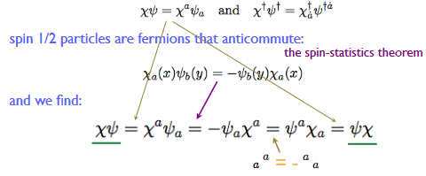
snippet grabbed from (Dermisek 09)
We analyze the special nature of the supergeometry space of field histories of the Dirac field a little (prop. 3.51) below and conclude by highlighting the crucial role of supergeometry (remark 3.52 below)
Proposition 3.51. (space of field histories of the Dirac field)
Let ##E = \Sigma \times S_{odd} \overset{pr_1}{\to} \Sigma## be the super-field bundle (def. 3.45) for the Dirac field over Minkowski spacetime ##\Sigma = \mathbb{R}^{p,1}## from example 3.50.
Then the corresponding supergeometric space of field histories
$$
\Gamma_\Sigma(\Sigma \times S_{odd})
\;\in\;
SuperSmoothSet
$$
from example 3.46 has the following properties:
- For ##U = \mathbb{R}^n## an ordinary Cartesian space (with no super-geometric thickening, def. 3.37) there is only a single ##U##-parameterized collection of field histories, hence a single plot$$
\Psi_{(-)}\;\colon\;\mathbb{R}^n \overset{ 0 }{\longrightarrow} \Gamma_\Sigma(\Sigma \times S_{odd})
$$and this corresponds to the zero section, hence to the trivial Dirac field$$
\Psi^A_{(-)} = 0
\,.
$$ - For ##U = \mathbb{R}^{n \vert 1}## a super Cartesian space (3.37) with a single super-odd dimension, then ##U##-parameterized collections of field histories$$
\Psi_{(-)} \;\colon\; \mathbb{R}^{n\vert 1} \longrightarrow \Gamma_\Sigma(\Sigma \times S_{odd})
$$are in natural bijection with plots of sections of the bosonic-field bundle with field fiber ##S_{even} = S## the spin representation regarded as an ordinary vector space:$$
\theta \Psi_{(-)} \;\colon\; \mathbb{R}^n \longrightarrow \Gamma_\Sigma(\Sigma \times S_{even})
\,,
$$
Moreover, these two kinds of plots determine the fermionic field space completely: It is in fact isomorphic, as a super vector space, to the bosonic field space shifted to odd degree (as in example 3.38):
$$
\Gamma_\Sigma(\Sigma \times S_{odd})
\;\simeq\;
\left(
\Gamma_\Sigma(E\times S_{even})
\right)_{odd}
\,.
$$
Proof. In the first case, the plot is a morphism of super Cartesian spaces (def. 3.37) of the form
$$
\mathbb{R}^n \times \mathbb{R}^{p,1} \longrightarrow S_{odd}
\,.
$$
By definitions, this is dually homomorphism of real supercommutative superalgebras
$$
C^\infty(\mathbb{R}^n \times \mathbb{R}^{p,1}) \longleftarrow \wedge^\bullet S^\ast
$$
from the Grassmann algebra on the
For the second case, notice that a morphism of the form
$$
\mathbb{R}^{n\vert 1}
\overset{\Psi_{(-)}}{\longrightarrow}
S_{odd}
$$
is by def. 3.48 naturally identified with a morphism of the form
$$
\mathbb{R}^n \overset{}{\longrightarrow} [\mathbb{R}^{0 \vert 1}, S_{odd}] \simeq S_{odd} \times S_{even}
\,,
$$
where the identification on the right is from example 3.49.
By the nature of Cartesian products, these morphisms, in turn, are naturally identified with pairs of morphisms of the form
$$
\left(
\array{
\mathbb{R}^n &\overset{}{\longrightarrow}& S_{odd}\,,
\\
\mathbb{R}^n &\overset{}{\longrightarrow}& S_{even}
}
\right)
\,.
$$
Now, as in the first point above, here, the first component is uniquely fixed to be the zero morphism ##\mathbb{R}^n \overset{0}{\to} S_{odd}##, and hence only the second component is free to choose. This is precisely the claim to be shown.
Remark 3.52. (supergeometric nature of the Dirac field)
Proposition 3.51 how two basic facts about the Dirac field, which may superficially seem to be in tension with each other, are properly unified by supergeometry:
- On the one hand, a field history ##\Psi## of the Dirac field is not an ordinary section of an ordinary vector bundle. In particular, its component functions ##\psi^A## anti-commute with each other, which is not the case for ordinary functions, and this is crucial for the Lagrangian density of the Dirac field to be well defined, we come to this below in example 5.8.
- On the other hand, a field history of the Dirac field is supposed to be a spinor, hence a section of a spinor bundle, which is an ordinary vector bundle.
Therefore prop. 3.51 serves to shows how, even though a Dirac field is not defined to be an ordinary section of an ordinary vector bundle, it is nevertheless encoded by such an ordinary section: One says that this ordinary section is a “superfield-component” of the Dirac field, the one linear in a Grassmann variable ##\theta##.
This concludes our discussion of the concept of fields itself. In the following chapter we consider the variational calculus of fields.
I am a researcher in the department Algebra, Geometry and Mathematical Physics of the Institute of Mathematics at the Czech Academy of the Sciences (CAS) in Prague.
Presently I am on leave at the Max Planck Institute for Mathematics in Bonn.


Leave a Reply
Want to join the discussion?Feel free to contribute!