
Learn Interacting Quantum Fields in Mathematical Quantum Field Theory
This is one chapter in a series on Mathematical Quantum Field Theory.
The previous chapter is 14. Free quantum fields.
The next chapter is 16. Renormalization.
15. Interacting quantum fields
In this chapter we discuss the following topics:
- Free field vacua
- Perturbative S-matrices
- Conceptual remarks
- Interacting field observables
- Time-ordered products
- (“Re”-)Normalization
- Feynman perturbation series
- Effective action
- Vacuum diagrams
- Interacting quantum BV-differential
- Ward identities
In the previous chapter we have found the quantization of free Lagrangian field theories by first choosing a gauge fixed BV-BRST-resolution of the algebra of gauge-invariant on-shell observables, then applying algebraic deformation quantization induced by the resulting Peierls-Poisson bracket on the graded covariant phase space to pass to a non-commutative algebra of quantum observables, such that, finally, the BV-BRST differential is respected.
Of course, most quantum field theories of interest are non-free; they are interacting field theories whose equations of motion is a non-linear differential equation. The archetypical example is the coupling of the Dirac field to the electromagnetic field via the electron-photon interaction, corresponding to the interacting field theory called quantum electrodynamics (discussed below).
In principle the perturbative quantization of such non-free field theory interacting field theories proceed the same way: One picks a BV-BRST-gauge fixing, computes the Peierls-Poisson bracket on the resulting covariant phase space (Khavkine 14), and then finds a formal deformation quantization of this Poisson structure to obtain the quantized non-commutative algebra of quantum observables, as formal power series in Planck’s constant ##\hbar##.
It turns out (Collini 16, Hawkins-Rejzner 16, prop. 15.25 below) that the resulting interacting formal deformation quantization may equivalently be expressed in terms of scattering amplitudes (example 15.12 below): These are the probability amplitudes for plane waves of free fields to come in from the far past, then interact in a compact region of spacetime via the given interaction (adiabatically switched-off outside that region) and emerge again as free fields into the far future.
The collection of all these scattering amplitudes, as the types and wave vectors of the incoming and outgoing free fields varies, is called the perturbative scattering matrix of the interacting field theory, or just S-matrix for short. It may equivalently be expressed as the exponential of time-ordered products of the adiabatically switched interaction action functional with itself (def. 15.3 below). The combinatorics of the terms in this exponential is captured by Feynman diagrams (prop. 15.51 below), which, with some care (remark 15.21 below), may be thought of as finite multigraphs (def. 15.50 below) whose edges are worldlines of virtual particles and whose vertices are the interactions that these particles undergo (def. 15.55 below).
The axiomatic definition of S-matrices for relativistic Lagrangian field theories and their rigorous construction via (“re”-)normalization of time-ordered products (def. 15.46 below) is called causal perturbation theory, due to (Epstein-Glaser 73). This makes precise and well-defined the would-be path integral quantization of interacting field theories (remark 15.16 below) and removes the errors (remark 15.19 below) and ensuing puzzlements (expressed in Feynman 85) that plagued the original informal conception of perturbative quantum field theory due to Schwinger-Tomonaga-Feynman-Dyson (remark 15.20 below).
The equivalent re-formulation of the formal deformation quantization of interacting field theories in terms of scattering amplitudes (prop. 15.25 below) has the advantage that it gives a direct handle on those observables that are measured in scattering experiments, such as the LHC experiment. The bulk of mankind’s knowledge about realistic perturbative quantum field theory — such as notably the standard model of particle physics — is reflected in such scattering amplitudes given via their Feynman perturbation series in formal powers of Planck’s constant and the coupling constant.
Moreover, the mathematical passage from scattering amplitudes to the actual interacting field algebra of quantum observables (def. 15.24 below) corresponding to the formal deformation quantization is well understood, given via “Bogoliubov’s formula” by the quantum Møller operators (def. 15.8 below).
Via Bogoliubov’s formula every perturbative S-matrix scheme (def. 15.3) induces for every choice of adiabatically switched interaction action functional a notion of perturbative interacting field observables (def. 15.8). These generate an algebra (def. 15.24 below). By Bogoliubov’s formula, in general, this algebra depends on the choice of adiabatic switching; which however is not meant to be part of the physics, but just a mathematical device for grasping global field structures locally.
But this spurious dependence goes away (prop. 15.27 below) when restricting attention to observables whose spacetime support is inside a compact causally closed subsets ##\mathcal{O}## of spacetime (def. 15.26 below). This is a sensible condition for an observable in physics, where any realistic experiment necessarily probes only a compact subset of spacetime, see also remark 15.18.
The resulting system (a “co-presheaf”) of well-defined perturbative interacting field algebras of observables (def. 15.29 below)
$$
\mathcal{O} \mapsto IntObs(E_{\text{BV-BRST}}, \mathbf{L}_{int})(\mathcal{O})
$$
is in fact causally local (prop. 15.30 below). This fact was presupposed without proof already in Il’in-Slavnov 78; because this is one of two key properties that the Haag-Kastler axioms (Haag-Kastler 64) demand of an intrinsically defined quantum field theory (i.e. defined without necessarily making recourse to the geometric backdrop of Lagrangian field theory). The only other key property demanded by the Haag-Kastler axioms is that the algebras of observables be C*-algebras; this however must be regarded as the axiom encoding non-perturbative quantum field theory and hence is necessarily violated in the present context of perturbative QFT.
Since quantum field theory following the full Haag-Kastler axioms is commonly known as AQFT, this perturbative version, with causally local nets of observables but without the C*-algebra-condition on them, has come to be called perturbative AQFT (Dütsch-Fredenhagen 01, Fredenhagen-Rejzner 12).
In this terminology the content of prop. 15.30 below is that while the input of causal perturbation theory is a gauge fixed Lagrangian field theory, the output is a perturbative algebraic quantum field theory:
$$
\array{
\array{
\text{gauge-fixed}
\\
\text{Lagrangian}
\\
\text{field theory}
}
&
\overset{
\array{
\text{causal}
\\
\text{perturbation theory}
\\
}
}{\longrightarrow}&
\array{
\text{perturbative}
\\
\text{algebraic}
\\
\text{quantum}
\\
\text{field theory}
}
\\
\underset{
\array{
\text{(Becchi-Rouet-Stora 76,}
\\
\text{Batalin-Vilkovisky 80s)}
}
}{\,}
&
\underset{
\array{
\text{(Bogoliubov-Shirkov 59,}
\\
\text{Epstein-Glaser 73)}
}
}{\,}
&
\underset{
\array{
\text{ (Il’in-Slavnov 78, }
\\
\text{Brunetti-Fredenhagen 99,}
\\
\text{Dütsch-Fredenhagen 01)}
}
}{\,}
}
$$
The independence of the causally local net of localized interacting field algebras of observables ##IntObs(E_{\text{BV-BRST}}, \mathbf{L}_{int} )(\mathcal{O})## from the choice of adiabatic switching implies a well-defined spacetime-global algebra of observables by forming the inductive limit
$$
IntObs(E_{\text{BV-BRST}}, \mathbf{L}_{int})
\;:=\;
\underset{\underset{\mathcal{O}}{\longrightarrow}}{\lim}
\left(
{\, \atop \,}
IntObs(E_{\text{BV-BRST}}, \mathbf{L}_{int})(\mathcal{O})
{\, \atop \,}
\right)
\,.
$$
This is also called the algebraic adiabatic limit, defining the algebras of observables of perturbative QFT “in the infrared”. The only remaining step in the construction of a perturbative QFT that remains is then to find an interacting vacuum state
$$
\left\langle
–
\right\rangle_{int}
\;\colon\;
IntObs(E_{\text{BV-BRST}}, \mathbf{L}_{int})
\longrightarrow
\mathbb{C}[ [ \hbar, g] ]
$$
on the global interacting field algebra ##Obs_{\mathbf{L}_{int}}##. This is related to the actual adiabatic limit, and it is by and large an open problem, see remark 15.18 below.
In conclusion, so far, the algebraic adiabatic limit yields, starting with a BV-BRST gauge fixed free field vacuum, the perturbative construction of interacting field algebras of observables (def. 15.24) and their organization in increasing powers of ##\hbar## and ##g## (loop order, prop. 15.68) via the Feynman perturbation series (example 15.58, example 15.71).
But this interacting field algebra of observables still involves all the auxiliary fields of the BV-BRST gauge fixed free field vacuum (as in example 15.54 for QED), while the actual physical gauge-invariant on-shell observables should be (just) the cochain cohomology of the BV-BRST differential on this enlarged space of observables. Hence for the construction of perturbative QFT to conclude, it remains to pass the BV-BRST differential of the free field Wick algebra of observables to a differential on the interacting field algebra, such that its cochain cohomology is well defined.
Since the time-ordered products away from coinciding interaction points are uniquely fixed (prop. 15.42 below), one finds that also this interacting quantum BV-differential is uniquely fixed, on regular polynomial observables, by conjugation with the quantum Møller operators (def. 15.72). The formula that characterizes it there is called the quantum master equation or equivalently the quantum master Ward identity (prop. 15.73 below).
In its incarnation as the master Ward identity, this expresses the difference between the shell of the free classical field theory and that of the interacting quantum field theory, thus generalizing the Schwinger-Dyson equation to interacting field theory (example 15.76 below). Applied to Noether’s theorem it expresses the possible failure of conserved currents associated with infinitesimal symmetries of the Lagrangian to still be conserved in the interacting perturbative QFT (example 15.78 below).
As one extends the time-ordered products to coinciding interaction points in (“re”-)normalization of the perturbative QFT (def. 15.46 below), the quantum master equation/master Ward identity becomes a renormalization condition (prop. 15.49 below). If this condition fails one says that the interacting perturbative QFT has a quantum anomaly, specifically a gauge anomaly if the Ward identity of an infinitesimal gauge symmetry is violated.
These issues of “(re)-“normalization we discuss in detail in the next chapter.
Free field vacua
In considering perturbative QFT, we are considering perturbation theory in formal deformation parameters around a fixed free Lagrangian quantum field theory in a chosen Hadamard vacuum state.
For convenient referencing we collect all the structure and notation that goes into this in the following definitions:
Definition 15.1. (free relativistic Lagrangian quantum field vacuum)
Let
- ##\Sigma## be a spacetime (e.g. Minkowski spacetime);
- ##(E,\mathbf{L})## a free Lagrangian field theory (def. 5.25), with field bundle ##E \overset{fb}{\to} \Sigma##;
- ##\mathcal{G} \overset{fb}{\to} \Sigma## a gauge parameter bundle for ##(E,\mathbf{L})## (def. 10.5), with induced BRST-reduced Lagrangian field theory ##\left( E \times_\Sigma \mathcal{G}[1], \mathbf{L} – \mathbf{L}_{BRST}\right)## (example 10.28);
- ##(E_{\text{BV-BRST}}, \mathbf{L}’ – \mathbf{L}’_{BRST})## a gauge fixing (def. 12.1) with graded BV-BRST field bundle ##E_{\text{BV-BRST}} = T^\ast_{\Sigma}[-1]\left( E\times_\Sigma \mathcal{G}[1] \times_\Sigma A \times_\Sigma A[-1]\right)## (remark 12.7);
- ##\Delta_H \in \Gamma'( E_{\text{BV-BRST}} \boxtimes E_{\text{BV-BRST}} )## a Wightman propagator ##\Delta_H = \tfrac{i}{2} \Delta + H## compatible with the causal propagator ##\Delta## which corresponds to the Green hyperbolic Euler-Lagrange equations of motion induced by the gauge-fixed Lagrangian density ##\mathbf{L}’##.
Given this, we write
$$
\left(
{\, \atop \,}
PolyObs(E_{\text{BV-BRST}})_{mc}[ [\hbar] ] \;,\;
\star_H
{\, \atop \,}
\right)
$$
for the corresponding Wick algebra-structure on formal power series in ##\hbar## (Planck’s constant) of microcausal polynomial observables (def. 14.2). This is a star algebra with respect to (coefficient-wise) complex conjugation (prop. 14.5).
Write
| $$ \label{HadamardVacuumStateForFreeFieldTheory} \array{ PolyObs(E_{\text{BV-BRST}})_{mc}[ [\hbar] ] &\overset{\langle – \rangle}{\longrightarrow}& \mathbb{C}[ [\hbar] ] \\ A &\mapsto& A(\Phi = 0) } $$ | (224) |
for the induced Hadamard vacuum state (prop. 14.15), hence the state whose distributional 2-point function is the chosen Wightman propagator:
$$
\left\langle \mathbf{\Phi}^a(x) \mathbf{\Phi}^b(y)\right\rangle
\;=\;
\hbar \, \Delta_H^{a b}(x,y)
\,.
$$
Given any microcausal polynomial observable ##A \in PolyObs(E_{\text{BV-BRST}})_{mc}[ [ \hbar, g, j] ]## then its value in this state is called its free vacuum expectation value
$$
\left\langle
A
\right\rangle
\;\in\;
\mathbb{C}[ [ \hbar, g, j] ]
\,.
$$
Write
| $$ \label{NormalOrderingLocalObservables} \array{ LocObs(E_{\text{BV-BRST}}) &\overset{\phantom{A}:(-):\phantom{A}}{\hookrightarrow}& PolyObs(E_{\text{BV-BRST}})_{mc} \\ A &\mapsto& :A: } $$ | (225) |
for the inclusion of local observables (def. 7.39) into microcausal polynomial observables (example 14.4), thought of as forming normal-ordered products in the Wick algebra (by def. 14.12).
We denote the Wick algebra-product (the star product ##\star_H## induced by the Wightman propagator ##\Delta_H## according to prop. 13.18) by juxtaposition (def. 14.12)
$$
A_1 A_2 \;:=\; A_1 \star_H A_2
\,.
$$
If an element ##A \in PolyObs(E_{\text{BV-BRST}})## has an inverse with respect to this product, we denote that by ##A^{-1}##:
$$
A^{-1} A = 1
\,.
$$
Finally, for ##A \in LocObs(E_{\text{BV-BRST}})## we write ##supp(A) \subset \Sigma## for its spacetime support (def. 7.31). For ##S_1, S_2 \subset \Sigma## two subsets of spacetime we write
$$
S_1 {\vee\!\!\!\wedge} S_2
\phantom{AAA}
\left\{
\array{
“S_1 \, \text{does not intersect the past of} \, S_2”
\\
\Updownarrow
\\
“S_2 \, \text{does not intersect the future of} \, S_1”
}
\right.
$$
for the causal order-relation (def. 2.37) and
$$
S_1 {\gt\!\!\!\!\lt} S_2
\phantom{AAA}
\text{for}
\phantom{AAA}
\array{
S_1 {\vee\!\!\!\wedge} S_2
\\
\text{and}
\\
S_2 {\vee\!\!\!\wedge} A_1
}
$$
for spacelike separation.
Being concerned with perturbation theory means mathematically that we consider formal power series in deformation parameters ##\hbar## (“Planck’s constant”) and ##g## (“coupling constant”), also in ##j## (“source field”), see also remark 15.14. The following collects our notational conventions for these matters:
Definition 15.2. (formal power series of observables for perturbative QFT)
Let ##(E_{\text{BV-BRST}}, \mathbf{L}’, \Delta_H )## be a relativistic free vacuum according to def. 15.1.
Write
$$
LocObs(E_{\text{BV-BRST}})[ [ \hbar, g, j ] ]
\;:=\;
\underset{ k_1, k_2, k_3 \in \mathbb{N}}{\prod}
LocObs(E_{\text{BV-BRST}})\langle \hbar^{k_1} g^{k_2} j^{k^3}\rangle
$$
for the space of formal power series in three formal variables
- ##\hbar## (“Planck’s constant”),
- ##g## (“coupling constant”)
- ##j## (“source field”)
with coefficients in the topological vector spaces of the off-shell polynomial local observables of the free field theory (def. 7.39); similarly for the off-shell microcausal polynomial observables (def. 14.2):
$$
PolyObs(E_{\text{BV-BRST}})_{mc}[ [ \hbar, g, j ] ]
\;:=\;
\underset{ k_1, k_2, k_3 \in \mathbb{N}}{\prod}
PolyObs(E_{\text{BV-BRST}})_{mc}\langle \hbar^{k_1} g^{k_2} j^{k^3}\rangle
\,.
$$
Similary
$$
LocObs(E_{\text{BV-BRST}})[ [ \hbar, g ] ]
\,,
\phantom{AAA}
PolyObs(E_{\text{BV-BRST}})[ [ \hbar, g ] ]
$$
denotes the subspace for which no powers of ##j## appear, etc.
Accordingly
$$
C^\infty_{cp}(\Sigma) \langle g \rangle
$$
denotes the vector space of bump functions on spacetime tensored with the vector space spanned by a single copy of ##g##. The elements
$$
g_{sw} \in C^\infty_{cp}(\Sigma)\langle g \rangle
$$
may be regarded as spacetime-dependent “coupling constants” with compact support, called adiabatically switched couplings.
Similarly then
$$
LocObs(E_{\text{BV-BRST}})[ [ \hbar, g, j ] ]\langle g , j \rangle
$$
is the subspace of those formal power series that are at least linear in ##g## or ##j## (hence those that vanish if one sets ##g,j = 0## ). Hence every element of this space may be written in the form
$$
O
=
g S_{int} + j A
\;\in\;
LocObs(E_{\text{BV-BRST}})[ [ \hbar, g, j ] ]\langle g , j \rangle
\,,
$$
where the notation is to suggest that we will think of the coefficient of ##g## as an (adiabatically switched) interaction action functional and of the coefficient of ##j## as an external source field (reflected by internal and external vertices, respectively, in Feynman diagrams, see def. 15.52 below).
In particular for
$$
\mathbf{L}_{int}
\;\in\;
\Omega^{p+1,0}_\Sigma(E_{\text{BV-BRST}})[ [ \hbar , g] ]
$$
a formal power series in ##\hbar## and ##g## of local Lagrangian densities (def. 5.1), thought of as a local interaction Lagrangians, and if
$$
g_{sw}
\;\in\;
C^\infty_{cp}(\Sigma) \langle g \rangle
$$
is an adiabatically switched coupling as before, then the transgression (def. 7.32) of the product
$$
g_{sw} \mathbf{L}_{int}
\;\in\;
\Omega^{p+1,0}_{\Sigma,cp}(E_{\text{BV-BRST}})[ [ \hbar ,g ] ]\langle g \rangle
$$
is such an adiabatically switched interaction
$$
g S_{int}
\;=\;
\tau_\Sigma( g_{sw} \mathbf{L}_{int} )
\;\in\;
LocObs(E_{\text{BV-BRST}})[ [ \hbar, g] ]\langle g \rangle
\,.
$$
We also consider the space of off-shell microcausal polynomial observables of the free field theory with formal parameters adjoined
$$
PolyObs(E_{\text{BV-BRST}})_{mc} ((\hbar)) [ [ g , j] ]
\,,
$$
which, in its ##\hbar##-dependent, is the space of Laurent series in ##\hbar##, hence the space exhibiting also negative formal powers of ##\hbar##.
Perturbative S-Matrices
We introduce now the axioms for perturbative scattering matrices relative to a fixed relativistic free Lagrangian quantum field vacuum (def. 15.1 below) according to causal perturbation theory (def. 15.3 below). Since the first of these axioms requires the S-matrix to be a formal sum of multi-linear continuous functionals, it is convenient to impose axioms on these directly: this is the axiomatics for time-ordered products in def. 15.31 below. That these latter axioms already imply the former is the statement of prop. 15.39, prop. 15.40 below . Its proof requires a close look at the “reverse-time ordered products” for the inverse S-matrix (def. 15.35 below) and their induced reverse-causal factorization (prop. 15.38 below).
Definition 15.3. (S-matrix axioms — causal perturbation theory)
Let ##(E_{\text{BV-BRST}}, \mathbf{L}’, \Delta_H )## be a relativistic free vacuum according to def. 15.1.
Then a perturbative S-matrix scheme for perturbative QFT around this free vacuum is a function
$$
\mathcal{S}
\;\;\colon\;\;
LocObs(E_{\text{BV-BRST}})[ [\hbar , g, j] ]\langle g, j \rangle
\overset{\phantom{AAA}}{\longrightarrow}
PolyObs(E_{\text{BV-BRST}})_{mc}((\hbar))[ [ g, j ] ]
$$
from local observables to microcausal polynomial observables of the free vacuum theory, with formal parameters adjoined as indicated (def. 15.2), such that the following two conditions “perturbation” and “causal additivity (jointly: “causal perturbation theory”) hold:
- (perturbation)There exist multi-linear continuous functionals (over ##\mathbb{C}[ [\hbar, g, j] ]##) of the form
$$
\label{TimeOrderedProductsInSMatrix}
T_k
\;\colon\;
\left(
{\, \atop \,}
LocObs(E_{\text{BV-BRST}})[ [\hbar, g, j] ]\langle g, j \rangle
{\, \atop \,}
\right)^{\otimes^k_{\mathbb{C}[ [\hbar, g, j] ]}}
\longrightarrow
PolyObs(E_{\text{BV-BRST}})_{mc}((\hbar))[ [ g, j ] ]
$$(226) for all ##k \in \mathbb{N}##, such that:
- The nullary map is constant on the unit of the Wick algebra$$
T_0( g S_{int} + j A) = 1
$$ - The unary map is the inclusion of local observables as normal-ordered products (225)$$
T_1(g S_{int} + j A) = g :S_{int}: + j :A:
$$ - The perturbative S-matrix is the exponential series of these maps in that for all ##g S_{int} + j A \in LocObs(E_{\text{BV-BRST}})[ [\hbar , g, j] ]\langle g,j\rangle ##
$$
\label{ExponentialSeriesScatteringMatrix}
\begin{aligned}
\mathcal{S}( g S_{int} + j A)
& =
T
\left(
\exp_{\otimes}
\left(
\tfrac{ 1 }{i \hbar}
\left(
g S_{int} + j A
\right)
\right)
\right)
\\
& :=
\underset{k = 0}{\overset{\infty}{\sum}}
\frac{1}{k!}
\left( \frac{1}{i \hbar} \right)^k
T_k
\left(
{\, \atop \,}
\underset{k\,\text{arguments}}{\underbrace{ (g S_{int} + jA) , \cdots, (g S_{int} + j A) }}
{\, \atop \,}
\right)
\end{aligned}
$$(227)
- The nullary map is constant on the unit of the Wick algebra$$
- (causal additivity)For all perturbative local observables ## O_0, O_1, O_2 \in LocObs(E_{\text{BV-BRST}})[ [\hbar, g, j] ]## we have
$$
\label{CausalAdditivity}
\left(
{\, \atop \,}
supp( O_1 ) {\vee\!\!\!\wedge} supp( O_2 )
{\, \atop \,}
\right)
\;\; \Rightarrow \;\;
\left(
{\, \atop \,}
\mathcal{S}( O_0 + O_1 + O_2 )
\;\,
\mathcal{S}( O_0 + O_1 )
\,
\mathcal{S}( O_0 )^{-1}
\,
\mathcal{S}(O_0 + O_2)
{\, \atop \,}
\right)
\,.
$$(228)
(The inverse ##\mathcal{S}(O)^{-1}## of ##\mathcal{S}(O)## with respect to the Wick algebra-structure is implied to exist by the axiom “perturbation”, see remark 15.4 below.)
Def. 15.3 is due to (Epstein-Glaser 73 (1)), following (Stückelberg 49-53, Bogoliubov-Shirkov 59). That the domain of an S-matrix scheme is indeed the space of local observables was made explicit (in terms of axioms for the time-ordered products, see def. 15.31 below), in (Brunetti-Fredenhagen 99, section 3, Dütsch-Fredenhagen 04, appendix E, Hollands-Wald 04,around (20)). The review includes (Rejzner 16, around def. 6.7, Dütsch 18, section 3.3).
Remark 15.4. (invertibility of the S-matrix)
The multiplicative inverse ##S(-)^{-1}## of the perturbative S-matrix in def. 15.3
with respect to the Wick algebra-product indeed exists, so that the list of axioms is indeed well defined: By the axiom “perturbation” this follows with the usual formula for the multiplicative inverse of formal power series that are non-vanishing in degree 0:
If we write
$$
\mathcal{S}(g S_{int} + j A) = 1 + \mathcal{D}(g S_{int} + j A)
$$
then
| $$ \label{InfverseOfPerturbativeSMatrix} \begin{aligned} \left( {\, \atop \,} \mathcal{S}(g S_{int} + j A) {\, \atop \,} \right)^{-1} &= \left( {\, \atop \,} 1 + \mathcal{D}(g S_{int} + j A) {\, \atop \,} \right)^{-1} \\ & = \underset{r = 0}{\overset{\infty}{\sum}} \left( {\, \atop \,} -\mathcal{D}(g S_{int} + j A) {\, \atop \,} \right)^r \end{aligned} $$ | (229) |
where the sum does exist in ##PolyObs(E_{\text{BV-BRST}})((\hbar))[ [[ g,j ] ]##, because (by the axiom “perturbation”) ##\mathcal{D}(g S_{int} + j A)## has vanishing coefficient in zeroth order in the formal parameters ##g## and ##j##, so that only a finite sub-sum of the formal infinite sum contributes in each order in ##g## and ##j##.
This expression for the inverse of S-matrix may usefully be re-organized in terms of “rever-time ordered products” (def. 15.35 below), see prop. 15.36 below.
Notice that ##\mathcal{S}(-g S_{int} – j A )## is instead the inverse with respect to the time-ordered products (226) in that
$$
T( \mathcal{S}(-g S_{int} – j A ) \,,\, \mathcal{S}(g S_{int} + j A) )
\;=\;
1
\;=\;
T( \mathcal{S}(g S_{int} + j A ) \,,\, \mathcal{S}(-g S_{in} – j A ) )
\,.
$$
(Since the time-ordered product is, by definition, symmetric in its arguments, the usual formula for the multiplicative inverse of an exponential series applies).
Remark 15.5. (adjoining further deformation parameters)
The definition of S-matrix schemes in def. 15.3 has immediate variants where arbitrary countable sets ##\{g_n\}## and ##\{j_m\}## of formal deformation parameters are considered, instead of just a single coupling constant ##g## and a single source field ##j##. The more such constants are considered, the “more perturbative” the theory becomes and the stronger the implications.
Given a perturbative S-matrix scheme (def. 15.3) it immediately induces a corresponding concept of observables:
Definition 15.6. (generating function scheme for interacting field observables)
Let ##(E_{\text{BV-BRST}}, \mathbf{L}’, \Delta_H )## be a relativistic free vacuum according to def. 15.1, let ##\mathcal{S}## be a corresponding S-matrix scheme according to def. 15.3.
The corresponding generating function scheme (for interacting field observables, def. 15.8 below) is the functional
$$
\mathcal{Z}_{(-)}(-)
\;\colon\;
LocObs(E_{\text{BV-BRST}})[ [\hbar, g] ]\langle g \rangle
\;\times\;
LocObs(E_{\text{BV-BRST}})[ [\hbar, j] ]\langle j \rangle
\longrightarrow
PolyObs(E_{\text{BV-BRST}})_{mc}((\hbar))[ [g , j] ]
$$
given by
| $$ \label{GeneratingFunctionInducedFromSMatrix} \mathcal{Z}_{g S_{int}}(j A) \;:=\; \mathcal{S}(g S_{int})^{-1} \mathcal{S}( g S_{int} + j A ) \,. $$ | (230) |
Proposition 15.7. (causal additivity in terms of generating functions)
In terms of the generating functions ##\mathcal{Z}## (def. 15.6) the axiom “causal additivity” on the S-matrix scheme ##\mathcal{S}## (def. 15.3) is equivalent to:
- (causal additivity in terms of ##\mathcal{Z}##)For all local observables ##O_0, O_1, O_2 \in LocObs(E_{\text{BV-BRST}})[ [\hbar, g, j] ]\otimes\mathbb{C}\langle g,j\rangle## we have
$$
\label{GeneratingFunctionCausalAdditivity}
\begin{aligned}
\left(
{\, \atop \,}
supp(O_1) {\vee\!\!\!\wedge} supp(O_2)
{\, \atop \,}
\right)
& \;\; \Rightarrow \;\;
\left(
{\, \atop \,}
\mathcal{Z}_{O_0}( O_1 ) \, \mathcal{Z}_{O_0}( O_2)
=
\mathcal{Z}_{ O_0 }( O_1 + O_2 )
{\, \atop \,}
\right)
\\
& \;\; \Leftrightarrow \;\;
\left(
{\, \atop \,}
\mathcal{Z}_{ O_0 + O_1 }( O_2 )
=
\mathcal{Z}_{ O_0 }( O_2 )
{\, \atop \,}
\right)
\end{aligned}
\,.
$$(231)
(Whence “additivity”.)
Proof. This follows by elementary manipulations:
Multiplying both sides of (228) by ##\mathcal{S}(O_0)^{-1}## yields
$$
\underset{
\mathcal{Z}_{ O_0 }( O_1 + O_2 )
}{
\underbrace{
\mathcal{S}( O_0 )^{-1}
\mathcal{S}( O_0 + O_1 + O_2 )
}
}
\;=\;
\underset{
\mathcal{Z}_{ O_0 }( O_1 )
}{
\underbrace{
\mathcal{S}( O_0 )^{-1} \mathcal{S}( O_0 + O_1 )
}
}
\underset{
\mathcal{Z}_{ O_0 }( O_2 )
}{
\underbrace{
\mathcal{S}( O_0 )^{-1} \mathcal{S}( O_0 + O_2 )
}
}
$$
This is the first line of (231).
Multiplying both sides of (228) by ##\mathcal{S}( O_0 + O_1 )^{-1}## yields
$$
\underset{
= \mathcal{Z}_{ O_0 + O_1 }( O_2 )
}{
\underbrace{
\mathcal{S}( O_0 + O_1 )^{-1}
\mathcal{S}( O_0 + O_1 + O_2 )
}
}
\;=\;
\underset{
= \mathcal{Z}_{ O_0 }( O_2 )
}{
\underbrace{
\mathcal{S}( O_0 )^{-1} \mathcal{S}( O_0 + O_2 )
}
}
\,.
$$
This is the second line of (231).
Definition 15.8. (interacting field observables — Bogoliubov’s formula)
Let ##(E_{\text{BV-BRST}}, \mathbf{L}’, \Delta_H )## be a relativistic free vacuum according to def. 15.1, let ##\mathcal{S}## be a corresponding S-matrix scheme according to def. 15.3, and let ##g S_{int} \in LocObs(E_{\text{BV-BRST}})[ [ \hbar, g ] ]\langle g \rangle## be a local observable regarded as an adiabatically switched interaction-functional.
Then for ##A \in LocObs(E_{\text{BV-BRST}})[ [\hbar , g] ]## a local observable of the free field theory, we say that the corresponding local interacting field observable
$$
A_{int} \in PolyObs(E_{\text{BV-BRST}})_{mc}[ [\hbar, g] ]
$$
is the coefficient of ##j^1## in the generating function (230):
| $$ \label{BogoliubovsFormula} \begin{aligned} A_{int} &:= i \hbar \frac{d}{d j} \left( {\, \atop \,} \mathcal{Z}_{ g S_{int} }( j A ) {\, \atop \,} \right)_{\vert_{j = 0}} \\ & := i \hbar \frac{d}{d j} \left( {\, \atop \,} \mathcal{S}(g S_{int})^{-1} \, \mathcal{S}( g S_{int} + j A ) {\, \atop \,} \right)_{\vert_{j = 0}} \\ & = \mathcal{S}(g S_{int})^{-1} T\left( \mathcal{S}(g S_{int}), A \right) \,. \end{aligned} $$ | (232) |
This expression is called Bogoliubov’s formula, due to (Bogoliubov-Shirkov 59).
One thinks of ##A_{int}## as the deformation of the local observable ##A## as the interaction ##S_{int}## is turned on, and speaks of an element of the interacting field algebra of observables. Their value (“expectation value”) in the given free Hadamard vacuum state ##\langle -\rangle## (def. 15.1) is a formal power series in Planck’s constant ##\hbar## and in the coupling constant ##g##, with coefficients in the complex numbers
$$
\left\langle
A_{int}
\right\rangle
\;\in\;
\mathbb{C}[ [\hbar, g] ]
$$
which express the probability amplitudes that reflect the predictions of the perturbative QFT, which may be compared to the experiment.
(Epstein-Glaser 73, around (74)); review includes (Dütsch-Fredenhagen 00, around (17), Dütsch 18, around (3.212)).
Remark 15.9. (interacting field observables are formal deformation quantization)
The interacting field observables in def. 15.8 are indeed formal power series in the formal parameter ##\hbar## (Planck’s constant), as opposed to being more general Laurent series, hence they involve no negative powers of ##\hbar## (Dütsch-Fredenhagen 00, prop. 2 (ii), Hawkins-Rejzner 16, cor. 5.2). This is not immediate, since by def. 15.3 the S-matrix that they are defined from does involve negative powers of ##\hbar##.
It follows in particular that the interacting field observables have a classical limit ##\hbar \to 0##, which is not the case for the S-matrix itself (due to it involving negative powers of ##\hbar##). Indeed the interacting field observables constitute a formal deformation quantization of the covariant phase space of the interacting field theory (prop. 15.25 below) and are thus the more fundamental concept.
As the name suggests, the S-matrices in def. 15.3 serve to express scattering amplitudes (example 15.12 below). But by remark 15.9
the more fundamental concept is that of the interacting field observables. Their perspective reveals that consistent interpretation of scattering amplitudes requires the following condition on the relation between the vacuum state and the interaction term:
Definition 15.10. (vacuum stability)
Let ##(E_{\text{BV-BRST}}, \mathbf{L}’, \Delta_H )## be a relativistic free vacuum according to def. 15.1, let ##\mathcal{S}## be a corresponding S-matrix scheme according to def. 15.3, and let ##g S_{int} \in LocObs(E_{\text{BV-BRST}})[ [ \hbar, g] ]\langle g \rangle## be a local observable, regarded as an adiabatically switched interaction action functional.
We say that the given Hadamard vacuum state (prop. 14.15)
$$
\langle – \rangle
\;\colon\;
PolyObs(E_{\text{BV-BRST}})_{mc}[ [ \hbar , g, j ] ]
\longrightarrow
\mathbb{C}[ [ \hbar, g, j ] ]
$$
is stable with respect to the interaction ##S_{int}##, if for all elements of the Wick algebra
$$
A \in PolyObs(E_{\text{BV-BRST}})_{mc}[ [ \hbar, g] ]
$$
we have
$$
\left\langle
A \mathcal{S}(g S_{int})
\right\rangle
\;=\;
\left\langle
\mathcal{S}(g S_{int})
\right\rangle
\,
\left\langle
A
\right\rangle
\phantom{AA}
\text{and}
\phantom{AA}
\left\langle
\mathcal{S}(g S_{int})^{-1}
A
\right\rangle
\;=\;
\frac{1}
{
\left\langle
\mathcal{S}(g S_{int})
\right\rangle
}
\left\langle
A
\right\rangle
$$
Example 15.11. (time-ordered product of interacting field observables)
Let ##(E_{\text{BV-BRST}}, \mathbf{L}’, \Delta_H )## be a relativistic free vacuum according to def. 15.1, let ##\mathcal{S}## be a corresponding S-matrix scheme according to def. 15.3, and let ##g S_{int} \in LocObs(E_{\text{BV-BRST}})[ [ \hbar, g ] ]\langle g \rangle## be a local observable regarded as an adiabatically switched interaction-functional.
Consider two local observables
$$
A_1, A_2
\;\in\;
LocObs(E_{\text{BV-BRST}})[ [ \hbar , g] ]
$$
with causally ordered spacetime support
$$
supp(A_1) {\vee\!\!\!\!\wedge} supp(A_2)
$$
Then causal additivity according to prop. 15.7 implies that the Wick algebra-product of the corresponding interacting field observables ##(A_1)_{int}, (A_2)_{int} \in PolyObs(E_{\text{BV-BRST}})[ [ \hbar, g ] ] ## (def. 15.8) is
$$
\begin{aligned}
(A_1)_{int}
(A_2)_{int}
& =
\left(
\frac{\partial}{\partial j} \mathcal{Z}(j A_1 )
\right)_{\vert j = 0}
\left(
\frac{\partial}{\partial j} \mathcal{Z}( j A_2 )
\right)_{\vert j = 0}
\\
& =
\frac{\partial^2}{\partial j_1 \partial j_2}
\left(
{\, \atop \,}
\mathcal{Z}( j_1 A_1 )
\mathcal{Z}( j_2 A_2 )
{\, \atop \,}
\right)_{
\left\vert { {j_1 = 0}, \atop {j_2 = 0} } \right.
}
\\
& =
\frac{\partial^2}{\partial j_1 \partial j_2}
\left(
{\, \atop \,}
\mathcal{Z}( j_1 A_1 + j_2 A_2 )
{\, \atop \,}
\right)_{
\left\vert { {j_1 = 0}, \atop {j_2 = 0} } \right.
}
\end{aligned}
$$
Here the last line makes sense if one extends the axioms on the S-matrix in prop. 15.3
from formal power series in ##\hbar, g, j## to formal power series in ##\hbar, g, j_1, j_2, \cdots## (remark 15.5). Hence in this generalization, the generating functions ##\mathcal{Z}## are not just generating functions for interacting field observables themselves, but in fact for time-ordered products of interacting field observables.
An important special case of time-ordered products of interacting field observables as in example 15.11
is the following special case of scattering amplitudes, which is the example that gives the scattering matrix in def. 15.3 its name:
Example 15.12. (scattering amplitudes as vacuum expectation values of interacting field observables)
Let ##(E_{\text{BV-BRST}}, \mathbf{L}’, \Delta_H )## be a relativistic free vacuum according to def. 15.1, let ##\mathcal{S}## be a corresponding S-matrix scheme according to def. 15.3, and let ##g S_{int} \in LocObs(E_{\text{BV-BRST}})[ [ \hbar, g ] ]\langle g \rangle## be a local observable regarded as an adiabatically switched interaction-functional, such that the vacuum state is stable with respect to ##g S_{int}## (def. 15.10).
Consider local observables
$$
\array{
A_{in,1}, \cdots, A_{in , n_{in}},
\\
A_{out,1}, \cdots, A_{out, n_{out}}
}
\;\;\in\;\;
LocObs(E_{\text{BV-BRST}})[ [ \hbar, g] ]
$$
whose spacetime support satisfies the following causal ordering:
$$
A_{out, i_{out} }
{\gt\!\!\!\!\lt}
A_{out, j_{out}}
\phantom{AAA}
A_{out, i_{out} }
{\vee\!\!\!\wedge}
S_{int}
{\vee\!\!\!\wedge}
A_{in, i_{in}}
\phantom{AAA}
A_{in, i_{in} }
{\gt\!\!\!\!\lt}
A_{in, j_{in}}
$$
for all ##1 \leq i_{out} \lt j_{out} \leq n_{out}## and ##1 \leq i_{in} \lt j_{in} \leq n_{in}##.
Then the vacuum expectation value of the Wick algebra product of the corresponding interacting field observables (def. 15.8) is
$$
\begin{aligned}
&
\left\langle
{\, \atop \,}
(A_{out, 1})_{int}
\cdots
(A_{out,n_{out}})_{int}
\,
(A_{in, 1})_{int}
\cdots
(A_{in,n_{in}})_{int}
{\, \atop \,}
\right\rangle
\\
& =
\left\langle
{\, \atop \,}
A_{out,1}
\cdots
A_{out,n_{out}}
\right|
\;
\mathcal{S}(g S_{int})
\;
\left|
A_{in,1}
\cdots
A_{in, n_{in}}
{\, \atop \,}
\right\rangle
\\
& :=
\frac{1}{
\left\langle \mathcal{S}(g S_{int}) \right\rangle
}
\left\langle
{\, \atop \,}
A_{out,1}
\cdots
A_{out,n_{out}}
\;
\mathcal{S}(g S_{int})
\;
A_{in,1}
\cdots
A_{in, n_{in}}
{\, \atop \,}
\right\rangle
\,.
\end{aligned}
$$
These vacuum expectation values are interpreted, in the adiabatic limit where ##g_{sw} \to 1##, as scattering amplitudes (remark 15.17 below).
Proof. For notational convenience, we spell out the argument for ##n_{in} = 1 = n_{out}##. The general case is directly analogous.
So assuming the causal order (def. 2.37)
$$
supp(A_{out})
{\vee\!\!\!\wedge}
supp(S_{int})
{\vee\!\!\!\wedge}
supp(A_{in})
$$
we compute with causal additivity via prop. 15.7 as follows:
$$
\begin{aligned}
(A_{out})_{int} (A_{in})_{int}
& =
\frac{d^2 }{\partial j_{out} \partial j_{in}}
\left(
\mathcal{Z}( j_{out} A_{out} )
\mathcal{Z}( j_{in} A_{in} )
\right)_{\left\vert { { j_{out} = 0 } \atop { j_{in} = 0 } } \right.}
\\
& =
\frac{\partial^2 }{\partial j_{out} \partial j_{in}}
\left(
\mathcal{S}(g S_{int})^{-1}
\underset{
=
\mathcal{S}(j_{out} A_{out})
\mathcal{S}(g S_{int})
}{
\underbrace{
\mathcal{S}(g S_{int} + j_{out} A_{out})
}
}
\mathcal{S}(g S_{int})^{-1}
\underset{
= \mathcal{S}(g S_{int}) \mathcal{S}(j_{in} A_{in})
}{
\underbrace{
\mathcal{S}(g S_{int} + j_{in}A_{in})
}
}
\right)_{\left\vert { { j_{out} = 0 } \atop { j_{in} = 0 } } \right.}
\\
& =
\frac{\partial^2 }{\partial j_{out} \partial j_{in}}
\left(
\mathcal{S}(g S_{int})^{-1}
\mathcal{S}(j_{out} A_{out})
\underset{
= \mathcal{S}(g S_{int})
}{
\underbrace{
\mathcal{S}(g S_{int})
\mathcal{S}(g S_{int})^{-1}
\mathcal{S}(g S_{int})
}
}
\mathcal{S}(j_{in} A_{in})
\right)_{\left\vert { { j_{out} = 0 } \atop { j_{in} = 0 } } \right.}
\\
& =
\mathcal{S}(g S_{int})^{-1}
\,
\left(
{\, \atop \,}
A_{out}
\mathcal{S}(g S_{int})
A_{in}
{\, \atop \,}
\right)
\,.
\end{aligned}
$$
With this the statement follows by the definition of vacuum stability (def. 15.10).
Remark 15.13. (computing S-matrices via Feynman perturbation series)
For practical computation of vacuum expectation values of interacting field observables (example 15.11) and hence in particular, via example 15.12, of scattering amplitudes, one needs some method for collecting all the contributions to the formal power series in increasing order in ##\hbar## and ##g##.
Such a method is provided by the Feynman perturbation series (example 15.58 below) and the effective action (def. 15.62), see example 15.71 below.
Conceptual remarks
The simple axioms for S-matrix schemes in causal perturbation theory (def. 15.3) and hence for interacting field observables (def. 15.8) have a wealth of implications and consequences. Before discussing these formally below, we here make a few informal remarks meant to put various relevant concepts into perspective:
Remark 15.14. (perturbative QFT and asymptotic expansion of probability amplitudes)
Given a perturbative S-matrix scheme (def. 15.3), then by remark 15.9 the expectation values of interacting field observables (def. 15.8) are formal power series in the formal parameters ##\hbar## and ##g## (which are interpreted as Planck’s constant, and as the coupling constant, respectively):
$$
\left\langle A_{int} \right\rangle
\;\in\;
\mathbb{C}[ [\hbar, g] ]
\,.
$$
This means that there is no guarantee that these series converge for any positive value of ##\hbar## and/or ##g##. In terms of synthetic differential geometry, this means that in perturbative QFT the deformation of the classical free field theory by quantum effects (measured by ##\hbar##) and interactions (measured by ##g##) is so very tiny as to actually be infinitesimal: formal power series may be read as functions on the infinitesimal neighborhood in a space of Lagrangian field theories at the point ##\hbar = 0##, ##g = 0##.
In fact, a simple argument (due to Dyson 52) suggests that in realistic field theories these series never converge for any positive value of ##\hbar## and/or ##g##. Namely convergence for ##g## would imply a positive radius of convergence around ##g = 0##, which would imply convergence also for ##-g## and even for imaginary values of ##g##, which would, however, correspond to unstable interactions for which no converging field theory is to be expected. (See Helling, p. 4 for the example of phi^4 theory.)
In physical practice, one tries to interpret these non-converging formal power series as asymptotic expansions of actual but hypothetical functions in ##\hbar, g##, which reflect the actual but hypothetical non-perturbative quantum field theory that one imagines is being approximated by perturbative QFT methods. An asymptotic expansion of a function is a power series that may not converge, but which has for every ##n \in \mathbb{N}## an estimate for how far the sum of the first ##n## terms in the series may differ from the function being approximated.
For examples such as quantum electrodynamics and quantum chromodynamics, as in the standard model of particle physics, the truncation of these formal power series scattering amplitudes to the first handful of loop orders in ##\hbar## happens to agree with experiment (such as at the LHC collider) to high precision (for QED) or at least decent precision (for QCD), at least away from infrared phenomena (see remark 15.18).
In summary, this says that perturbative QFT is an extremely coarse and restrictive approximation to what should be genuine non-perturbative quantum field theory, while at the same time it happens to match certain experimental observations to a remarkable degree, albeit only if some ad-hoc truncation of the resulting power series is considered.
This is a strong motivation for going beyond perturbative QFT to understand and construct genuine non-perturbative quantum field theory. Unfortunately, this is a wide-open problem, away from toy examples. Not a single interacting field theory in spacetime dimension ##\geq 4## has been non-perturbatively quantized. Already a single aspect of the non-perturbative quantization of Yang-Mills theory (as in QCD) has famously been advertised as one of the Millenium Problems of our age; and speculation about non-perturbative quantum gravity is the subject of much activity.
Now, as the name indicates, the axioms of causal perturbation theory (def. 15.3) do not address non-perturbative aspects of non-perturbative field theory; the convergence or non-convergence of the formal power series that are axiomatized by Bogoliubov’s formula (def. 15.8) is not addressed by the theory. The point of the axioms of causal perturbation theory is to give rigorous mathematical meaning to everything else in perturbative QFT.
Remark 15.15. (Dyson series and Schrödinger equation in interaction picture)
The axiom “causal additivity” (228) on an S-matrix scheme (def. 15.3) implies immediately this seemingly weaker condition (which turns out to be equivalent, this is prop. 15.40 below):
- (causal factorization)For all local observables ##O_1, O_2 \in LocObs(E_{\text{BV-BRST}})[ [\hbar, h, j] ]\langle g , j\rangle ## we have$$
\left(
{\, \atop \,}
supp(O_1) {\vee\!\!\!\wedge} supp(O_2)
{\, \atop \,}
\right)
\;\; \Rightarrow \;\;
\left(
{\, \atop \,}
\mathcal{S}( O_1 + O_2 )
=
\mathcal{S}( O_1 ) \, \mathcal{S}( O_2 )
{\, \atop \,}
\right)
$$
(This is the special case of “causal additivity” for ##O_0 = 0##, using that by the axiom “perturbation” (227) we have ##\mathcal{S}(0) = 1##.)
If we now think of ##O_1 = g S_{1}## and ##O_2 = g S_2## themselves as adiabatically switched interaction action functionals, then this becomes
$$
\left(
{\, \atop \,}
supp(S_1) {\vee\!\!\!\wedge} supp(S_2)
{\, \atop \,}
\right)
\;\; \Rightarrow \;\;
\left(
{\, \atop \,}
\mathcal{S}( g S_1 + g S_2 )
=
\mathcal{S}( g S_1) \, \mathcal{S}( g sS_2)
{\, \atop \,}
\right)
$$
This exhibits the S-matrix-scheme as a “causally ordered exponential” or “Dyson series” of the interaction, hence as a refinement to the relativistic field theory of what in quantum mechanics is the “integral version of the Schrödinger equation in the interaction picture” (see this equation at S-matrix; see also Scharf 95, the second half of 0.3).
The relevance of manifest causal additivity of the S-matrix, over just causal factorization (even though both conditions happen to be equivalent, see prop. 15.40 below), is that it directly implies that the induced interacting field algebra of observables (def. 15.8) forms a causally local net (prop. 15.30 below).
Remark 15.16. (path integral-intuition)
In the informal discussion of perturbative QFT going back to informal ideas of Schwinger-Tomonaga-Feynman-Dyson, the perturbative S-matrix is thought of in terms of a would-be path integral, symbolically written
$$
\mathcal{S}\left(
g S_{int} + j A
\right)
\;\overset{\text{not really!}}{=}\;
\!\!\!\!\!
\underset{\Phi \in \Gamma_\Sigma(E_{\text{BV-BRST}})_{asm}}{\int}
\!\!\!\!\!\!
\exp\left(
\tfrac{1}{i \hbar}
\int_\Sigma
\left(
g L_{int}(\Phi) + j A(\Phi)
\right)
\right)
\,
\exp\left(
\tfrac{1}{i \hbar}\int_\Sigma L_{free}(\Phi)
\right) D[\Phi]
\,.
$$
Here the would-be integration is thought to be over the space of field histories ##\Gamma_\Sigma(E_{\text{BV-BRST}})_{asm}## (the space of sections of the given field bundle) for field histories which satisfy given asymptotic conditions at ##x^0 \to \pm \infty##; and as these boundary conditions vary the above is regarded as a would-be integral kernel that defines the required operator in the Wick algebra (e.g. Weinberg 95, around (9.3.10) and (9.4.1)). This is related to the intuitive picture of the Feynman perturbation series expressing a sum over all possible interactions of virtual particles (remark 15.21).
Beyond toy examples, it is not known how to define the would-be measure ##D[\Phi]## and it is not known how to make sense of this expression as an actual integral.
The analogous path-integral intuition for Bogoliubov’s formula for interacting field observables (def. 15.8) symbolically reads
$$
\begin{aligned}
A_{int}
& \overset{\text{not really!}}{=}
\frac{d}{d j}
\ln
\left(
\underset{\Phi \in \Gamma_\Sigma(E)_{asm}}{\int}
\!\!\!\!
\exp\left(
\underset{\Sigma}{\int}
g L_{int}(\Phi) + j A(\Phi)
\right)
\,
\exp\left( \underset{\Sigma}{\int} L_{free}(\Phi) \right)
D[\Phi]
\right)
\vert_{j = 0}
\end{aligned}
$$
If here we were to regard the expression
$$
\mu(\Phi)
\;\overset{\text{not really!}}{:=}\;
\frac{
\exp\left( \underset{\Sigma}{\int} L_{free}(\Phi) \right)\, D[\Phi]
}
{
\underset{\Phi \in \Gamma_\Sigma(E_{\text{BV-BRST}})_{asm}}{\int}
\!\!\!\!
\exp\left( \underset{\Sigma}{\int} L_{free}(\Phi) \right)\, D[\Phi]
}
$$
as a would-be Gaussian measure on the space of field histories, normalized to a would-be probability measure, then this formula would express interacting field observables as ordinary expectation values
$$
A_{int}
\overset{\text{not really!}}{=}
\!\!\!
\underset{\Phi \in \Gamma_\Sigma(E_{\text{BV-BRST}})_{asm}}{\int}
\!\!\!\!\!\!
A(\Phi)
\,\mu(\Phi)
\,.
$$
As before, beyond toy examples, it is not known how to make sense of this as an actual integration.
But we may think of the axioms for the S-matrix in causal perturbation theory (def. 15.3) as rigorously defining the path integral, not analytically as an actual integration, but synthetically by axiomatizing the properties of the desired outcome of the would-be integration:
The analogy with a well-defined integral and the usual properties of an exponential vividly suggest that the would-be path integral should obey causal factorization. Instead of trying to make sense of path integration so that this factorization property could then be appealed to as a consequence of general properties of integration and exponentials, the axioms of causal perturbation theory directly prescribe the desired factorization property, without insisting that it derives from an actual integration.
The great success of path integral-intuition in the development of quantum field theory, despite the dearth of actual constructions, indicates that it is not the would-be integration process as such that actually matters in field theory, but only the resulting properties that this suggests the S-matrix should have; which is what causal perturbation theory axiomatizes. Indeed, the simple axioms of causal perturbation theory rigorously imply finitely (i.e. (“re”-)normalized) perturbative quantum field theory (see remark 15.20).
$$
\array{
\array{
\text{would-be}
\\
\text{path integral}
\\
\text{intuition}
}
&
\overset{
\array{
\text{informally}
\\
\text{suggests}
}
}{\longrightarrow}
&
\array{
\text{causally additive}
\\
\text{scattering matrix}
}
&
\overset{
\array{
\text{rigorously}
\\
\text{implies}
}
}{\longrightarrow}
&
\array{
\text{UV-finite}
\\
\text{(i.e. (re-)normalized)}
\\
\text{perturbative QFT}
}
}
$$
Remark 15.17. (scattering amplitudes)
Let ##(E_{\text{BV-BRST}}, \mathbf{L}’, \Delta_H )## be a relativistic free vacuum according to def. 15.1, let ##\mathcal{S}## be a corresponding S-matrix scheme according to def. 15.3, and let
$$
S_{int} \in LocObs(E_{\text{BV-BRST}})[ [ \hbar, g ] ]
$$
be a local observable, regarded as an adiabatically switched interaction action functional.
Then for
$$
A_{in}, A_{out} \in PolyObs(E_{\text{BV-BRST}})_{mc}[ [\hbar] ]
$$
two microcausal polynomial observables, with causal ordering
$$
supp(A_{out}) {\vee\!\!\!\wedge} supp(A_{int})
$$
the corresponding scattering amplitude (as in example 15.12) is the value (called “expectation value” when referring to ##A^\ast_{out} \, \mathcal{S}(S_{int}) \, A_{in}##, or “matrix element” when referring to ##\mathcal{S}(S_{int})##, or “transition amplitude” when referring to ##\left\langle A_{out} \right\vert## and ##\left\vert A_{in} \right\rangle##)
$$
\left\langle
A_{out}
\,\vert\,
\mathcal{S}(S_{int})
\,\vert\,
A_{in}
\right\rangle
\;:=\;
\left\langle
A^\ast_{out} \, \mathcal{S}(S_{int}) \, A_{in}
\right\rangle
\;\in\;
\mathbb{C}[ [ \hbar, g ] ]
\,.
$$
for the Wick algebra-product ##A^\ast_{out} \, \mathcal{S}(S_{int})\, A_{in} \in PolyObs(E_{\text{BV-BRST}})[ [\hbar, g ] ]## in the given Hadamard vacuum state ##\langle -\rangle \colon PolyObs(E_{\text{BV-BRST}})[ [\hbar, g] ] \to \mathbb{C}[ [\hbar,g] ]##.
If here ##A_{in}## and ##A_{out}## are monomials in Wick algebra-products of the field observables ##\mathbf{\Phi}^a(x) \in Obs(E_{\text{BV-BRST}})[ [\hbar] ]##, then this scattering amplitude comes from the integral kernel
$$
\begin{aligned}
&
\left\langle
\mathbf{\Phi}^{a_{out,1}}(x_{out,1}) \cdots \mathbf{\Phi}^{a_{out,s}}(x_{out,s})
\vert
\,
\mathcal{S}(S_{int})
\,
\vert
\mathbf{\Phi}^{a_{in,1}}(x_{in,1})
\cdots
\mathbf{\Phi}^{a_{in,r}}(x_{in,r})
\right\rangle
\\
& :=
\left\langle
\left(\mathbf{\Phi}^{a_{out,1}}(x_{out,1})\right)^\ast
\cdots
\left(\mathbf{\Phi}^{a_{out,s}}(x_{out,s})\right)^\ast
\;\mathcal{S}(S_{int})\;
\mathbf{\Phi}^{a_{in,1}}(x_{in,1})
\cdots
\mathbf{\Phi}^{a_{in,r}}(x_{in,r})
\right\rangle
\end{aligned}
$$
or similarly, under Fourier transform of distributions,
| $$ \label{ScatteringPlaneWaves} \begin{aligned} & \left\langle \widehat{\mathbf{\Phi}}^{a_{out,1}}(k_{out,1}) \cdots \widehat{\mathbf{\Phi}}^{a_{out,s}}(k_{out,s}) \vert \, \mathcal{S}(S_{int}) \, \vert \widehat{\mathbf{\Phi}}^{a_{in,1}}(k_{in,1}) \cdots \widehat{\mathbf{\Phi}}^{a_{in,r}}(k_{in,r}) \right\rangle \\ & := \left\langle \left(\widehat{\mathbf{\Phi}}^{a_{out,1}}(k_{out,1})\right)^\ast \cdots \left(\widehat{\mathbf{\Phi}}^{a_{out,s}}(k_{out,s})\right)^\ast \;\mathcal{S}(S_{int})\; \widehat{\mathbf{\Phi}}^{a_{in,1}}(k_{in,1}) \cdots \widehat{\mathbf{\Phi}}^{a_{in,r}}(k_{in,r}) \right\rangle \end{aligned} \,. $$ | (233) |
These are interpreted as the (distributional) probability amplitudes for plane waves of field species ##a_{in,\cdot}## with wave vector ##k_{in,\cdot}## to come in from the far past, ineract with each other via ##S_{int}##, and emerge in the far future as plane waves of field species ##a_{out,\cdot}## with wave vectors ##k_{out,\cdot}##.
Or rather:
Remark 15.18. (adiabatic limit, infrared divergences, and interacting vacuum)
Since a local observable ##S_{int} \in LocObs(E_{\text{BV-BRST}})[ [\hbar, g, j] ]## by definition has compact spacetime support, the scattering amplitudes in remark 15.17
describe scattering processes for interactions that vanish (are “adiabatically switched off”) outside a compact subset of spacetime. This constraint is crucial for causal perturbation theory to work.
There are several aspects to this:
- (adiabatic limit) On the one hand, real physical interactions ##\mathbf{L}_{int}## (say the electron-photon interaction) are not really supposed to vanish outside a compact region of spacetime. In order to reflect this mathematically, one may consider a sequence of adiabatic switchings ##g_{sw} \in C^\infty_{cp}(\Sigma)\langle g \rangle## (each of compact support) whose limit is the constant function ##g \in C^\infty(\Sigma)\langle g\rangle## (the actual coupling constant), then consider the corresponding sequence of interaction action functionals ##S_{int,sw} := \tau_\Sigma( g_{sw} \mathbf{L}_{int} )## and finally consider:
- as the true scattering amplitude the corresponding limit$$
\left\langle
A_{out} \vert \mathcal{S}(S_{int}) \vert A_{int}
\right\rangle
\;:=\;
\underset{g_{sw} \to 1}{\lim}
\left\langle
A_{out} \vert \mathcal{S}(S_{int,sw}) \vert A_{int}
\right\rangle
$$of adiabatically switched scattering amplitudes (remark 15.17) — if it exists. This is called the strong adiabatic limit.
- as the true n-point functions the corresponding limit$$
\begin{aligned}
&
\left\langle
\mathbf{\Phi}^{a_1}_{int}(x_1)
\mathbf{\Phi}^{a_2}_{int}(x_2)
\cdots
\mathbf{\Phi}^{a_{n-1}}_{int}(x_{n-1})
\mathbf{\Phi}^{a_n}_{int,sw}(x_n)
\right\rangle
\\
& =
\underset{\underset{g_{sw} \to 1}{\longrightarrow}}{\lim}
\left\langle
\mathbf{\Phi}^{a_1}_{int,sw}(x_1)
\mathbf{\Phi}^{a_2}_{int,sw}(x_2)
\cdots
\mathbf{\Phi}^{a_{n-1}}_{int,sw}(x_{n-1})
\mathbf{\Phi}^{a_n}_{int,sw}(x_n)
\right\rangle
\end{aligned}
$$of tempered distributional expectation values of products of interacting field observables (def. 15.8) — if it exists. (Similarly for time-ordered products.) This is called the weak adiabatic limit.
Beware that the left-hand sides here are symbolic: Even if the limit exists in expectation values, in general, there is no actual observable whose expectation value is that limit.
The strong and weak adiabatic limits have been shown to exist if all fields are massive (Epstein-Glaser 73). The weak adiabatic limit has been shown to exists for quantum electrodynamics and for mass-less phi^4 theory (Blanchard-Seneor 75) and for larger classes of field theories in (Duch 17, p. 113, 114).
If these limits do not exist, one says that the perturbative QFT has an infrared divergence.
- as the true scattering amplitude the corresponding limit$$
- (algebraic adiabatic limit) On the other hand, it is equally unrealistic that an actual experiment detects phenomena outside a given compact subset of spacetime. Realistic scattering experiments (such as the LHC) do not really prepare or measure plane waves filling all of the spacetime as described by the scattering amplitudes (233). Any observable that is realistically measurable must-have compact spacetime support. We see below in prop. 15.27 that such interacting field observables with compact spacetime support may be computed without taking the adiabatic limit: It is sufficient to use any adiabatic switching which is constant on the support of the observable. This way one obtains for each causally closed subset ##\mathcal{O}## of spacetime an algebra of observables ##\mathcal{A}_{int}(\mathcal{O})## whose support is in ##\mathcal{O}##, and for each inclusion of subsets a corresponding inclusion of algebras of observables (prop. 15.30 below). Of this system of observables, one may form the category-theoretic inductive limit to obtain a single global algebra of observables.$$
\mathcal{A}_{int}
\;:=\;
\underset{\underset{\mathcal{O}}{\longrightarrow}}{\lim}
\mathcal{A}_{int}(\mathcal{O})
$$This always exists. It is called the algebraic adiabatic limit (going back to Brunetti-Fredenhagen 00, section 8).For quantum electrodynamics the algebraic adiabatic limit was worked out in (Dütsch-Fredenhagen 98, reviewed in Dütsch 18, 5,3). - (interacting vacuum) While, via the above algebraic adiabatic limit, causal perturbation theory yields the correct interacting field algebra of quantum observables independent of choices of adiabatic switching, a theory of quantum probability requires, on top of the algebra of observables, also a state$$
\langle – \rangle_{int} \;\colon\; \mathcal{A}_{int} \longrightarrow \mathbb{C}[ [\hbar] ]
$$Just as the interacting field algebra of observables ##\mathcal{A}_{int}## is a deformation of the free field algebra of observables (Wick algebra), there ought to be a corresponding deformation of the free Hadamard vacuum state ##\langle- \rangle## into an “interacting vacuum state” ##\langle – \rangle_{int}##. Sometimes the weak adiabatic limit serves to define the interacting vacuum (see Duch 17, p. 113-114).
A stark example of these infrared issues is the phenomenon of confinement of quarks to hadron bound states (notably to protons and neutrons) at large wavelengths. This is paramount in observation and reproduced in numerical lattice gauge theory simulation, but is invisible to perturbative quantum chromodynamics in its free field vacuum state, due to infrared divergences. It is expected that this should be rectified by the proper interacting vacuum of QCD (Rafelski 90, pages 12-16), which is possibly a “theta-vacuum” exhibiting superposition of QCD instantons (Schäfer-Shuryak 98, section III.D). This remains open, closely related to the Millenium Problem of quantization of Yang-Mills theory.
In contrast to the above subtleties about the infrared divergences, any would-be UV-divergences in perturbative QFT are dealt with by causal perturbation theory:
Remark 15.19. (the traditional error leading to UV-divergences)
Naively it might seem that (say over Minkowski spacetime, for simplicity) examples of time-ordered products according to def. 15.31
might simply be obtained by multiplying Wick algebra-products with step functions ##\Theta## of the time coordinates, hence to write, in the notation as generalized functions (remark 15.33):
$$
T(x_1, x_2)
\overset{\text{no!}}{=}
\Theta(x_1^0 – x_2^0) \, T(x_1) \, T(x_2)
+
\Theta(x_2^0 – x_1^0) \, T(x_2) \, T(x_1)
$$
and analogously for time-ordered products of more arguments (for instance Weinberg 95, p. 143, between (3.5.9) and (3.5.10)).
This however is simply a mathematical error (as amplified in Scharf 95, below (3.2.4), below (3.2.44), and in fig. 3):
Both ##T## as well as ##\Theta## are distributions and their product of distributions is in general not defined, as Hörmander’s criterion (prop. 9.34), which is exactly what guarantees the absence of UV-divergences (remark 9.27), may be violated. The notorious ultraviolet divergences which plagued (Feynman 85) the original conception of perturbative QFT due to Schwinger-Tomonaga-Feynman-Dyson are the signature of this ill-defined product (see remark 15.20).
On the other hand, when both distributions are restricted to the complement of the diagonal (i.e. restricted away from coinciding points ##x_1 = x_2##), then the step function becomes a non-singular distribution so that the above expression happens to be well defined and does solve the axioms for time-ordered products.
Hence what needs to be done to properly define the time-ordered product is to choose an extension of distributions of the above product expression back from the complement of the diagonal to the whole space of tuples of points. Any such extension will produce time-ordered products.
There are in general several different such extensions. This freedom of choice is the freedom of “re-” normalization; or equivalently, by the main theorem of perturbative renormalization theory (theorem 16.19 below), this is the freedom of choosing “counterterms” (remark 16.24 below) for the local interactions. This we discuss below and in more detail in the next chapter.
Remark 15.20. (absence of ultraviolet divergences and re-normalization)
The simple axioms of causal perturbation theory (def. 15.3) do fully capture perturbative quantum field theory “in the ultraviolet”: A solution to these axioms induces, by definition, well-defined perturbative scattering amplitudes (remark 15.17) and well-defined perturbative probability amplitudes of interacting field observables (def. 15.8) induced by local action functionals (describing point-interactions such as the electron-photon interaction). By the main theorem of perturbative renormalization (theorem 16.19) such solutions exist. This means that, while these are necessarily formal power series in ##\hbar## and ##g## (remark 15.14), all the coefficients of these formal power series (“loop order contributions”) are well defined.
This is in contrast to the original informal conception of perturbative QFT due to Schwinger-Tomonaga-Feynman-Dyson, which is a first stage produced ill-defined diverging expressions for the coefficients (due to the mathematical error discussed in remark 15.19 below), which were then “re-normalized” to finite values, by further informal arguments.
Here in causal perturbation theory, no divergences in the coefficients of the formal power series are considered in the first place, all coefficients are well-defined, hence “finite”. In this sense, causal perturbation theory is about “finite” perturbative QFT, where instead of “re-normalization” of ill-defined expressions one just encounters “normalization” (prominently highlighted in Scharf 95, see the title, introduction, and section 4.3), namely compatible choices of these finite values. The actual “re-normalization” in the sense of “change of normalization” is expressed by the Stückelberg-Petermann renormalization group.
This refers to those divergences that are known as UV-divergences, namely short-distance effects, which are mathematically reflected in the fact that the perturbative S-matrix scheme (def. 15.3) is defined on local observables, which, by their very locality, encode point-interactions. See also remark 15.18 on infrared divergences.
Remark 15.21. (virtual particles, worldline formalism, and perturbative string theory)
It is suggestive to think of the edges in the Feynman diagrams (def. 15.55) as worldlines of “virtual particles” and of the vertices as the points where they collide and transmute. (Care must be exercised not to confuse this with concepts of real particles.) With this interpretation prop. 15.56 may be read as saying that the scattering amplitude for given external source fields (remark 15.17) is the superposition of the Feynman amplitudes of all possible ways that these may interact; which is closely related to the intuition for the path integral (remark 15.16).
This intuition is made precise by the worldline formalism of perturbative quantum field theory (Strassler 92). This is the perspective on perturbative QFT which directly relates perturbative QFT to perturbative string theory (Schmidt-Schubert 94). In fact, the worldline formalism for perturbative QFT was originally found by taking the point-particle limit of string scattering amplitudes (Bern-Kosower 91, Bern-Kosower 92).
Remark 15.22. (renormalization scheme)
Beware the terminology in def. 15.3: A single S-matrix is one single observable
$$
\mathcal{S}(S_{int})
\;\in\;
PolyObs(E_{\text{BV-BRST}})_{mc}((\hbar))[ [g,j] ]
$$
for a fixed (adiabatically switched local) interaction ##S_{int}##, reflecting the scattering amplitudes (remark 15.17) with respect to that particular interaction. Hence the function
$$
\mathcal{S}
\;\colon\;
LocObs(E_{\text{BV-BRST}})[ [\hbar, g,j] ]\langle g, j
\rangle
\longrightarrow
PolyObs(E_{\text{BV-BRST}})((\hbar))[ [g,j] ]
$$
axiomatized in def. 15.3 is really a whole scheme for constructing compatible S-matrices for all possible (adiabatically switched, local) interactions at once.
Since the usual proof of the construction of such schemes of S-matrices involves (“re”-)normalization, the function ##\mathcal{S}## axiomatized by def. 15.3 may also be referred to as a (“re”-)normalization scheme.
This perspective on ##\mathcal{S}## as a renormalization scheme is amplified by the main theorem of perturbative renormalization (theorem 16.19) which states that the space of choices for ##\mathcal{S}## is a torsor over the Stückelberg-Petermann renormalization group.
Remark 15.23. (quantum anomalies)
The axioms for the S-matrix in def. 15.3
(and similarly that for the time-ordered products below in def. 15.31) are sufficient to imply a causally local net of perturbative interacting field algebras of quantum observables (prop. 15.30 below), and thus its algebraic adiabatic limit (remark 15.18).
It does not guarantee, however, that the BV-BRST differential passes to those algebras of quantum observables, hence it does not guarantee that the infinitesimal symmetries of the Lagrangian are respected by the quantization process (there may be “quantum anomalies”). The extra condition that does ensure this is the quantum master Ward identity or quantum master equation. This we discuss elsewhere.
Apart from gauge symmetries one also wants to require that rigid symmetries are preserved by the S-matrix, notably Poincare group-symmetry for scattering on Minkowski spacetime.
Interacting field observables
We now discuss how the perturbative interacting field observables that are induced from an S-matrix enjoy good properties expected of any abstractly defined perturbative algebraic quantum field theory.
Definition 15.24. (interacting field algebra of observables — quantum Møller operator)
Let ##(E_{\text{BV-BRST}}, \mathbf{L}’, \Delta_H )## be a relativistic free vacuum according to def. 15.1, let ##\mathcal{S}## be a corresponding S-matrix scheme according to def. 15.3, and let ##g S_{int} \in LocObs(E_{\text{BV-BRST}})[ [ \hbar, g ] ]## be a local observable regarded as an adiabatically switched interaction-functional.
We write
$$
LocIntObs_{\mathcal{S}}(E_{\text{BV-BRST}}, g S_{int})
\;:=\;
\left\{
{\, \atop \,}
A_{int} \;\vert\; A \in LocObs(E_{BV-BRST})[ [ \hbar, g ] ]
{\, \atop \,}
\right\}
\hookrightarrow
PolyObs(E_{\text{BV-BRST}})[ [ \hbar, g] ]
$$
for the subspace of interacting field observables ##A_{int}## (def. 15.8) corresponding to local observables ##A##, the local interacting field observables.
Furthermore, we write
$$
\array{
LocObs(E_{\text{BV-BRST}})[ [ \hbar , g] ]
&
\underset{\simeq}{\overset{\phantom{A}\mathcal{R}^{-1}\phantom{A}}{\longrightarrow}}
&
IntLocObs(E_{\text{BV-BRST}}, g S_{int})[ [ \hbar , g ] ]
\\
A
&\mapsto&
A_{int}
:=
\mathcal{S}(g S_{int})^{-1} T( \mathcal{S}(g S_{int}), A )
}
$$
for the factorization of the function ##A \mapsto A_{int}## through its image, which, by remark 15.4, is a linear isomorphism with inverse
$$
\array{
IntLocObs(E_{\text{BV-BRST}}, g S_{int})[ [ \hbar , g ] ]
&
\underset{\simeq}{\overset{\phantom{A}\mathcal{R}\phantom{A}}{\longrightarrow}}
&
LocObs(E_{\text{BV-BRST}})[ [ \hbar , g] ]
\\
A_{int}
&\mapsto&
A
:=
T\left(
\mathcal{S}(-g S_{int})
,
\left( \mathcal{S}(g S_{int}) A_{int} \right)
\right)
}
$$
This may be called the quantum Møller operator (Hawkins-Rejzner 16, (33)).
Finally, we write
$$
\begin{aligned}
IntObs(E_{\text{BV-BRST}}, S_{int})
& :=
\left\langle
{\, \atop \,}
IntLocObs(E_{\text{BV-BRST}})[ [ \hbar, g] ]
{\, \atop \,}
\right\rangle
\\
&
\phantom{:=}
\hookrightarrow
PolyObs(E_{\text{BV-BRST}})[ [ \hbar, g ] ]
\end{aligned}
$$
for the smallest subalgebra of the Wick algebra containing the interacting local observables. This is the perturbative interacting field algebra of observables.
The definition of the interacting field algebra of observables from the data of a scattering matrix (def. 15.3) via Bogoliubov’s formula (def. 15.8) is physically well-motivated but is not immediately recognizable as the result of applying a systematic concept of quantization (such as formal deformation quantization) to the given Lagrangian field theory. The following proposition 15.25 says that this is nevertheless the case. (The special case of this statement for free field theory is discussed at Wick algebra, see remark 14.6).
Proposition 15.25. (interacting field algebra of observables is formal deformation quantization of interacting Lagrangian field theory)
Let ##(E_{\text{BV-BRST}}, \mathbf{L}’, \Delta_H )## be a relativistic free vacuum according to def. 15.1, and let ##g_{sw} \mathbf{L}_{int} \in \Omega^{p+1,0}_{\Sigma,cp}(E_{\text{BV-BRST}})[ [\hbar, g ] ]\langle g\rangle## be an adiabatically switched interaction Lagrangian density with corresponding action functional ##g S_{int} := \tau_\Sigma( g_{sw} \mathbf{L}_{int} )##.
Then, at least on regular polynomial observables, the construction of perturbative interacting field algebras of observables in def. 15.24 is a formal deformation quantization of the interacting Lagrangian field theory ##(E_{\text{BV-BRST}}, \mathbf{L}’ + g_{sw} \mathbf{L}_{int})##.
(Hawkins-Rejzner 16, prop. 5.4, Collini 16)
The following definition collects the system (a co-presheaf) of generating functions for interacting field observables which are localized in spacetime as the spacetime localization region varies:
Definition 15.26. (system of spacetime-localized generating functions for interacting field observables)
Let ##(E_{\text{BV-BRST}}, \mathbf{L}’, \Delta_H )## be a relativistic free vacuum according to def. 15.1, let ##\mathcal{S}## be a corresponding S-matrix scheme according to def. 15.3, and let
$$
\mathbf{L}_{int}
\;\in\;
\Omega^{p+1,0}_\Sigma(E_{\text{BV-BRST}})[ [ \hbar , g ] ]
$$
be a Lagrangian density, to be thought of as an interaction, so that for ##g_{sw} \in C^\infty_{sp}(\Sigma)\langle g \rangle## an adiabatic switching the transgression
$$
S_{int,sw}
\;:=\;
\tau_\Sigma(g_{sw} \mathbf{L}_{int})
\;\in\;
LocObs(E_{\text{BV-BRST}})[ [ \hbar, g, j] ]
$$
is a local observable, to be thought of as an adiabatically switched interaction action functional.
For ##\mathcal{O} \subset \Sigma## a causally closed subset of spacetime (def. 2.38) and for ##g_{sw} \in Cutoffs(\mathcal{O})## an adiabatic switching function (def. 2.39) which is constant on a neighbourhood of ##\mathcal{O}##, write
$$
Gen(E_{\text{BV-BRST}}, S_{int,sw} )(\mathcal{O})
\;:=\;
\left\langle
\mathcal{Z}_{S_{int,sw}}(j A)
\;\vert\;
A \in LocObs(E_{\text{BV-BRST}})[ [ \hbar, g] ]
\,\text{with}\,
supp(A) \subset \mathcal{O}
\right\rangle
\;\subset\;
PolyObs(E_{\text{BV-BRST}})[ [ \hbar, g, j] ]
$$
for the smallest subalgebra of the Wick algebra which contains the generating functions (def. 15.6) with respect to ##S_{int,sw}## for all those local observables ##A## whose spacetime support is in ##\mathcal{O}##.
Moreover, write
$$
Gen(E_{\text{BV-BRST}}, \mathbf{L}_{int})(\mathcal{O})
\;\subset\;
\underset{g_{sw} \in Cutoffs(\mathcal{O})}{\prod}
Gen(E_{\text{BV-BRST}}, S_{int,sw})(\mathcal{O})
$$
be the subalgebra of the Cartesian product of all these algebras as ##g_{sw}## ranges over cutoffs, which is generated by the tuples
$$
\mathcal{Z}_{\mathbf{L}_{int}}(A)
\;:=\;
\left(
\mathcal{Z}_{S_{int,sw}}(j A)
\right)_{g_{sw} \in Cutoffs(\mathcal{O})}
$$
for ##A## with ##supp(A) \subset \mathcal{O}##.
We call ##Gen(E_{\text{BV-BRST}}, \mathbf{L}_{int} )(\mathcal{O})## the algebra of generating functions for interacting field observables localized in ##\mathcal{O}##.
Finally, for ##\mathcal{O}_1 \subset \mathcal{O}_2## an inclusion of two causally closed subsets, let
$$
i_{\mathcal{O}_1, \mathcal{O}_2}
\;\colon\;
Gen(E_{\text{BV-BRST}}, \mathbf{L}_{int})(\mathcal{O}_1)
\longrightarrow
Gen(E_{\text{BV-BRST}}, \mathbf{L}_{int})(\mathcal{O}_2)
$$
be the algebra homomorphism which is given simply by restricting the index set of tuples.
This construction defines a functor
$$
Gen(E_{\text{BV-BRST}}, \mathbf{L}_{int})
\;\colon\;
CausClsdSubsets(\Sigma)
\longrightarrow
Algebras
$$
from the poset of causally closed subsets of spacetime to the category of algebras.
(extends to star algebras if scattering matrices are chosen unitary…)
(Brunetti-Fredenhagen 99, (65)-(67))
The key technical fact is the following:
Proposition 15.27. (localized interacting field observables independent of adiabatic switching)
Let ##(E_{\text{BV-BRST}}, \mathbf{L}’, \Delta_H )## be a relativistic free vacuum according to def. 15.1, let ##\mathcal{S}## be a corresponding S-matrix scheme according to def. 15.3, and let
$$
\mathbf{L}_{int}
\;\in\;
\Omega^{p+1,0}_\Sigma(E_{\text{BV-BRST}})[ [ \hbar , g ] ]
$$
be a Lagrangian density, to be thought of as an interaction, so that for ##g_{sw} \in C^\infty_{sp}(\Sigma)\langle g \rangle## an adiabatic switching the transgression
$$
g S_{int,sw} \;:=\; \tau_\Sigma(g_{sw} \mathbf{L}_{int})
\;\in\;
LocObs(E_{\text{BV-BRST}})[ [ \hbar, g, j] ]
$$
is a local observable, to be thought of as an adiabatically switched interaction action functional.
If two such adiabatic switchings ##g_{sw,1}, g_{sw,2} \in C^\infty_{cp}(\Sigma)## agree on a causally closed subset
$$
\mathcal{O} \;\subset\; \Sigma
$$
in that
$$
g_{sw,1}\vert_{\mathcal{O}} = g_{sw,2}\vert_{\mathcal{O}}
$$
then there exists a microcausal polynomial observable
$$
K \;\in\; PolyObs(E_{\text{BV-BRST}})_{mc}[ [ \hbar, g, j ] ]
$$
such that for every local observable
$$
A \;\in\; LocObs(E_{\text{BV-BRST}})[ [ \hbar, g ] ]
$$
with spacetime support in ##\mathcal{O}##
$$
supp(A) \;\subset\; \mathcal{O}
$$
the corresponding two generating functions (230) are related via conjugation by ##K##:
| $$ \label{AdiabaticSwitchingRelationGeneratingFunctions} \mathcal{Z}_{S_{int,sw_2}} \left( j A \right) \;=\; K^{-1} \, \left( \mathcal{Z}_{S_{int,sw_1}} \left( j A \right) \right) \, K \,. $$ | (234) |
In particular this means that for every choice of adiabatic switching ##g_{sw} \in Cutoffs(\mathcal{O})## the algebra ##Gen_{S_{int,sw}}(\mathcal{O})## of generating functions for interacting field observables computed with ##g_{sw}## is canonically isomorphic to the abstract algebra ##Gen_{\mathbf{L}_{int}}(\mathcal{O})## (def. 15.26), by the evident map on generators:
| $$ \label{AbstractGeneratingFunctionAlgebraIsomorphicToAnyAdiabaticSwitching} \array{ Gen(E_{\text{BV-BRST}}, \mathbf{L}_{int})(\mathcal{o}) &\overset{\simeq}{\longrightarrow}& Gen(E_{\text{BV-BRST}}, S_{int,sw})(\mathcal{O}) \\ \left( \mathcal{Z}_{S_{int,sw’}} \right)_{g_{sw’} \in Cutoffs(\mathcal{O})} &\mapsto& \mathcal{Z}_{S_{int,sw}} } \,. $$ | (235) |
(Brunetti-Fredenhagen 99, prop. 8.1)
Proof. By causal closure of ##\mathcal{O}##, lemma 2.40
says that there are bump functions
$$
a, r \in C^\infty_{cp}(\Sigma)\langle g \rangle
$$
which decompose the difference of adiabatic switchings
$$
g_{sw,2} – g_{sw,1} = a + r
$$
subject to the causal ordering
$$
supp(a) \,{\vee\!\!\!\wedge}\, \mathcal{O} \,{\vee\!\!\!\wedge}\, supp(r)
\,.
$$
With this the result follows from repeated use of causal additivity in its various equivalent incarnations from prop. 15.7:
$$
\begin{aligned}
& \mathcal{Z}_{g S_{int,sw_2}}(j A)
\\
& =
\mathcal{Z}_{
\left(
\tau_\Sigma
\left(
g_{sw,2}
\mathbf{L}_{int}
\right)
\right)
}
\left(
j A
\right)
\\
& =
\mathcal{Z}_{
\left(
\tau_\Sigma
\left(
(g_{sw,1} + a + r)\mathbf{L}_{int}
\right)
\right)
}
\left(
j A
\right)
\\
& =
\mathcal{Z}_{
\left(
g S_{int,sw_1}
+
\tau_\Sigma
\left(
r \mathbf{L}_{int}
\right)
+
\tau_\Sigma
\left(
a \mathbf{L}_{int}
\right)
\right)
}
\left(
j A
\right)
\\
& =
\mathcal{Z}_{
\left(
g S_{int,sw_1}
+
\tau_\Sigma
\left(
r \mathbf{L}_{int}
\right)
\right)
}
\left(
j A
\right)
\\
& =
\mathcal{S}
\left(
g S_{int,sw_1}
+
\tau_\Sigma
\left(
r \mathbf{L}_{int}
\right)
\right)^{-1}
\,
\mathcal{S}
\left(
g S_{int,sw_1}
+
j A
+
\tau_\Sigma
\left(
r \mathbf{L}_{int}
\right)
\right)
\\
& =
\mathcal{S}
\left(
g S_{int,sw_1}
+
\tau_\Sigma
\left(
r \mathbf{L}_{int}
\right)
\right)^{-1}
\,
\mathcal{S}
\left(
g S_{int,sw_1}
+
j A
\right)
\,
\mathcal{S}
\left(
g S_{int,sw_1}
\right)^{-1}
\,
\mathcal{S}
\left(
j A
+
\tau_\Sigma
\left(
r \mathbf{L}_{int}
\right)
\right)
\\
& =
\mathcal{S}
\left(
g S_{int,sw_1}
+
\tau_\Sigma
\left(
r\mathbf{L}_{int}
\right)
\right)^{-1}
\,
\underset{
= id
}{
\underbrace{
\mathcal{S}
\left(
g S_{int,sw_1}
\right)
\,
\mathcal{S}
\left(
g S_{int,sw_1}
\right)^{-1}
}
}
\,
\mathcal{S}
\left(
g S_{int,sw_1}
+
j A
\right)
\,
\mathcal{S}
\left(
g S_{int , sw_1}
\right)^{-1}
\,
\mathcal{S}
\left(
j A
+
\tau_\Sigma
\left(
r \mathbf{L}_{int}
\right)
\right)
\\
& =
\underset{
K^{-1}
}{
\underbrace{
\left(
\mathcal{Z}_{
g S_{int,sw_1}
}
\left(
\tau_\Sigma
\left(
r \mathbf{L}_{int}
\right)
\right)
\right)^{-1}
}
}
\,
\mathcal{Z}_{
g S_{int,sw_1}
}
\left(
j A
\right)
\,\,
\underset{
K
}{
\underbrace{
\mathcal{Z}_{
g S_{int,sw_1}
}
\left(
\tau_\Sigma
\left(
r \mathbf{L}_{int}
\right)
\right)
}}
\end{aligned}
$$
This proves the existence of elements ##K## as claimed.
It is clear that conjugation induces an algebra homomorphism, and since the map is a linear isomorphism on the space of generators, it is an algebra isomorphism on the algebras being generated (235).
(While the elements ##K## in (234) are far from being unique themselves, equation (234) says that the map on generators induced by conjugation with ##K## is independent of this choice.)
Proposition 15.28. (system of generating algebras is causally local net)
Let ##(E_{\text{BV-BRST}}, \mathbf{L}’, \Delta_H )## be a relativistic free vacuum according to def. 15.1, let ##\mathcal{S}## be a corresponding S-matrix scheme according to def. 15.3, and let
$$
\mathbf{L}_{int}
\;\in\;
\Omega^{p+1,0}_\Sigma(E_{\text{BV-BRST}})[ [ \hbar , g ] ]
$$
be a Lagrangian density, to be thought of as an interaction.
Then the system
$$
Gen(E_{\text{BV-BRST}}, \mathbf{L}_{int})
\;\colon\;
CausCldSubsets(\Sigma)
\longrightarrow
Algebra
$$
of localized generating functions for interacting field observables (def. 15.26) is a causally local net in that it satisfies the following conditions:
- (isotony) For every inclusion ##\mathcal{O}_1 \subset \mathcal{O}_2## of causally closed subsets of spacetime the corresponding algebra homomorphism is a monomorphism$$
i_{\mathcal{O}_1, \mathcal{O}_2}
\;\colon\;
Gen(E_{\text{BV-BRST}}, \mathbf{L}_{int})(\mathcal{O}_1) \hookrightarrow Gen(E_{\text{BV-BRST}},\mathbf{L}_{int})(\mathcal{O}_2)
$$ - (causal locality) For ##\mathcal{O}_1, \mathcal{O}_2 \subset X## two causally closed subsets which are spacelike separated, in that their causal ordering (def. 2.37) satisfies$$
\mathcal{O}_1 {\vee\!\!\!\wedge} \mathcal{O}_2
\;\text{and}\;
\mathcal{O}_2 {\vee\!\!\!\wedge} \mathcal{O}_1
$$and for ##\mathcal{O} \subset \Sigma## any further causally closed subset which contains both$$
\mathcal{O}_1 , \mathcal{O}_2 \subset \mathcal{O}
$$then the corresponding images of the generating function algebras of interacting field observables localized in ##\mathcal{O}_1## and in ##\mathcal{O}_2##, respectively, commute with each other as subalgebras of the generating function algebras of interacting field observables localized in ##\mathcal{O}##:$$
\left[
i_{\mathcal{O}_1,\mathcal{O}}(Gen_{L_{int}}(\mathcal{O}_1))
\;,\;
i_{\mathcal{O}_2,\mathcal{O}}(Gen_{L_{int}}(\mathcal{O}_2))
\right]
\;=\;
0
\;\;\;
\in Gen(E_{\text{BV-BRST}}, \mathbf{L}_{int})(\mathcal{O})
\,.
$$
(Dütsch-Fredenhagen 00, section 3, following Brunetti-Fredenhagen 99, section 8, Il’in-Slavnov 78)
Proof. Isotony is immediate from the definition of the algebra homomorphisms in def. 15.26.
By the isomorphism (235) we may check causal locality with respect to any choice of adiabatic switching ##g_{sw} \in Cautoff(\mathcal{O})## constant over ##\mathcal{O}##. For this the statement follows, with the assumption of spacelike separation, by causal additivity (prop. 15.7):
For ##supp(A_1) \subset \mathcal{O}_1## and ##supp(A_2) \subset \mathcal{O}_2## we have:
$$
\begin{aligned}
\mathcal{Z}_{g S_{int,sw}}( j A_1 )
\mathcal{Z}_{g S_{int,sw}}( j A_2 )
& =
\mathcal{S}_{g S_{int,sw}}( j A_1 + j A_2)
\\
& =
\mathcal{S}_{g S_{int,sw}}( j A_2 + j A_1)
\\
& =
\mathcal{Z}_{g S_{int,sw}}( j A_2 )
\mathcal{Z}_{g S_{int,sw}}( j A_1 )
\end{aligned}
$$
With the causally local net of localized generating functions for interacting field observables in hand, it is now immediately to get the
Definition 15.29. (system of interacting field algebras of observables)
Let ##(E_{\text{BV-BRST}}, \mathbf{L}’, \Delta_H )## be a relativistic free vacuum according to def. 15.1, let ##\mathcal{S}## be a corresponding S-matrix scheme according to def. 15.3, and let
$$
\mathbf{L}_{int}
\;\in\;
\Omega^{p+1,0}_\Sigma(E_{\text{BV-BRST}})[ [ \hbar , g ] ]
$$
be a Lagrangian density, to be thought of as an interaction, so that for ##g_{sw} \in C^\infty_{sp}(\Sigma)\langle g \rangle## an adiabatic switching the transgression
$$
g S_{int,sw} \;:=\; g \tau_\Sigma(g_{sw} \mathbf{L}_{int})
\;\in\;
LocObs(E_{\text{BV-BRST}})[ [ \hbar, g ] ]\langle g \rangle
$$
is a local observable, to be thought of as an adiabatically switched interaction action functional.
For ##\mathcal{O} \subset \Sigma## a causally closed subset of spacetime (def. 2.38) and for ##g_{sw} \in Cutoffs(\mathcal{O})## an compatible adiabatic switching function (def. 2.39) write
$$
IntObs(E_{\text{BV-BRST}}, S_{int,sw})(\mathcal{O})
:=
\left\langle
i \hbar \frac{d}{d j}
\mathcal{Z}_{S_{int}}(j A)\vert_{j = 0} \;\vert\; supp(A) \subset \mathcal{O}
\right\rangle
\;\subset\;
PolyObs((\hbar))[ [ g ] ]
$$
for the interacting field algebra of observables (def. 15.24) with spacetime support in ##\mathcal{O}##.
Let then
$$
IntObs(E_{\text{BV-BRST}}, \mathbf{L}_{int})(\mathcal{O})
\subset
\underset{g_{sw} \in Cutoffs(\mathcal{O})}{\prod} IntObs(E_{\text{BV-BRST}}, S_{int,sw})(\mathcal{O})
$$
be the subalgebra of the Cartesian product of all these algebras as ##g_{sw}## ranges, which is generated by the tuples
$$
i \hbar
\frac{d}{d j } \mathcal{Z}_{\mathbf{L}_{int}}\vert_{j = 0}
\;:=\;
\left(
i \hbar
\frac{d}{d j } \mathcal{Z}_{S_{int,sw}} (j A)\vert_{j = 0}
\right)_{g_{sw} \in Cutoffs(\mathcal{O})}
$$
for ##supp(A) \subset \mathcal{O}##.
Finally, for ##\mathcal{O}_1 \subset \mathcal{O}_2## an inclusion of two causally closed subsets, let
$$
i_{\mathcal{O}_1, \mathcal{O}_2}
\;\colon\;
IntObs(E_{\text{BV-BRST}}, \mathbf{L}_{int})(\mathcal{O}_1)
\longrightarrow
IntObs(E_{\text{BV-BRST}}, \mathbf{L}_{int})(\mathcal{O}_2)
$$
be the algebra homomorphism which is given simply by restricting the index set of tuples.
This construction defines a functor
$$
IntObs(E_{\text{BV-BRST}}, \mathbf{L}_{int}) \;\colon\; CausClsdSubsets(\Sigma) \longrightarrow Algebras
$$
from the poset of causally closed subsets in the spacetime ##\Sigma## to the category of star algebras.
Finally, as a direct corollary of prop. 15.28, we obtain the key result:
Proposition 15.30. (system of interacting field algebras of observables is causally local)
Let ##(E_{\text{BV-BRST}}, \mathbf{L}’, \Delta_H )## be a relativistic free vacuum according to def. 15.1, let ##\mathcal{S}## be a corresponding S-matrix scheme according to def. 15.3, and let
$$
\mathbf{L}_{int}
\;\in\;
\Omega^{p+1,0}_\Sigma(E_{\text{BV-BRST}})[ [ \hbar , g ] ]
\,.
$$
be a Lagrangian density, to be thought of as an interaction, then the system of algebras of observables ##Obs_{L_{int}}## (def. 15.29) is a local net of observables in that
- (isotony) For every inclusion ##\mathcal{O}_1 \subset \mathcal{O}_2## of causally closed subsets the corresponding algebra homomorphism is a monomorphism$$
i_{\mathcal{O}_1, \mathcal{O}_2}
\;\colon\;
IntObs(E_{\text{BV-BRST}}, \mathbf{L}_{int})(\mathcal{O}_1) \hookrightarrow IntObs(E_{\text{BV-BRST}}, \mathbf{L}_{int})(\mathcal{O}_2)
$$ - (causal locality) For ##\mathcal{O}_1, \mathcal{O}_2 \subset X## two causally closed subsets which are spacelike separated, in that their causal ordering (def. 2.37) satisfies$$
\mathcal{O}_1 {\vee\!\!\!\wedge} \mathcal{O}_2
\;\text{and}\;
\mathcal{O}_2 {\vee\!\!\!\wedge} \mathcal{O}_1
$$and for ##\mathcal{O} \subset \Sigma## any further causally closed subset which contains both$$
\mathcal{O}_1 , \mathcal{O}_2 \subset \mathcal{O}
$$then the corresponding images of the generating algebras of ##\mathcal{O}_1## and ##\mathcal{O}_2##, respectively, commute with each other as subalgebras of the generating algebra of ##\mathcal{O}##:$$
\left[
i_{\mathcal{O}_1,\mathcal{O}}(Obs_{\mathbf{L}_{int}}(\mathcal{O}_1))
\;,\;
i_{\mathcal{O}_2,\mathcal{O}}(Obs_{\mathbf{L}_{int}}(\mathcal{O}_2))
\right]
\;=\;
0
\;\;\;
\in IntObs(E_{\text{BV-BRST}}, \mathbf{L}_{int})(\mathcal{O})
\,.
$$
(Dütsch-Fredenhagen 00, below (17), following Brunetti-Fredenhagen 99, section 8, Il’in-Slavnov 78)
Proof. The first point is again immediate from the definition (def. 15.29).
For the second point, it is sufficient to check the commutativity relation on generators. For these, the statement follows with prop. 15.28:
$$
\begin{aligned}
& \left[
i \hbar \frac{d}{d j} \mathcal{Z}_{S_{int,sw}}(j A_1)\vert_{j = 0}
\;,\;
i \hbar \frac{d}{d j} \mathcal{Z}_{S_{int,sw}}(j J_2)\vert_{j = 0}
\right]
\\
& =
(i \hbar)^2
\frac{
\partial^2
}{
\partial j_1 \partial j_2
}
\underset{ = 0}{
\underbrace{
\left[
\mathcal{Z}_{S_{int,sw}}(j_1 A_1)
\;,\;
\mathcal{Z}_{S_{int,sw}}(j_1 A_2)
\right]}}_{ \left\vert { {j_1 = 0} \atop {j_2 = 0} } \right. }
\\
& = 0
\end{aligned}
$$
time-ordered products
Definition 15.3 suggests focusing on the multilinear operations ##T(…)## which define the perturbative S-matrix order-by-order in ##\hbar##. We impose axioms on these time-ordered products directly (def. 15.31) and then prove that these axioms imply the axioms for the corresponding S-matrix (prop. 15.39 below).
Definition 15.31. (time-ordered products)
Let ##(E_{\text{BV-BRST}}, \mathbf{L}’, \Delta_H )## be a free vacuum according to def. 15.1.
A time-ordered product is a sequence of multi-linear continuous functionals for all ##k \in \mathbb{N}## of the form
$$
T_k
\;\colon\;
\left(
{\, \atop \,}
LocObs(E_{\text{BV-BRST}})[ [\hbar, g, j] ]\langle g,j \rangle
{\, \atop \,}
\right)^{\otimes^k_{\mathbb{C}[ [\hbar, g, j] ]}}
\longrightarrow
PolyObs(E_{\text{BV-BRST}})_{reg}((\hbar))[ [g , j] ]
$$
(from tensor products of local observables to microcausal polynomial observables, with formal parameters adjoined according to def. 15.2) such that the following conditions hold for all possible arguments:
- (normalization)$$
T_0(O) = 1
$$ - (perturbation)$$
T_1(O) = :O:
$$ - (symmetry) each ##T_k## is symmetric in its arguments, in that for every permutation ##\sigma \in \Sigma(k)## of ##k## elements$$
T_k(O_{\sigma(1)}, O_{\sigma(2)}, \cdots, O_{\sigma(k)})
\;=\;
T_k(O_1, O_2, \cdots, O_k)
$$ - (causal factorization) If the spacetime support (def. 7.31) of local observables satisfies the causal ordering (def. 2.37)$$
\left(
{\, \atop \,}
supp(O_1)
\cup
\cdots
\cup
supp(O_r)
{\, \atop \,}
\right)
\;{\vee\!\!\!\wedge}\;
\left(
{\, \atop \,}
supp(O_{r+1})
\cup
\cdots
\cup
supp(O_k)
{\, \atop \,}
\right)
$$then the time-ordered product of these ##k## arguments factors as the Wick algebra-product of the time-ordered product of the first ##r## and that of the second ##k-r## arguments:$$
T(O_1, \cdots, O_k)
\; = \;
T( O_1, \cdots , O_r )
\,
T( O_{r+1}, \cdots , O_k )
\,.
$$
Example 15.32. (S-matrix scheme implies time-ordered products)
Let ##(E_{\text{BV-BRST}}, \mathbf{L}’, \Delta_H )## be a relativistic free vacuum according to def. 15.1 and let
$$
\mathcal{S}
\;=\;
\underset{k \in \mathbb{N}}{\sum}
\frac{1}{k!}\frac{1}{(i \hbar)^k}
T_k
$$
be a corresponding S-matrix scheme according to def. 15.3.
Then the ##\{T_k\}_{k \in \mathbb{N}}## are time-ordered products in the sense of def. 15.31.
Proof. We need to show that the ##\{T_k\}_{k \in \mathbb{N}}## satisfy causal factorization.
For
$$
O_j\;\in\; LocObs(E_{\text{BV-BRST}})[ [ \hbar, g, j] ]\langle g,j\rangle
$$
a local observable, consider the continuous linear function that multiplies this by any real number
$$
\array{
\mathbb{R}
&\longrightarrow&
LocObs(E_{\text{BV-BRST}})[ [ \hbar, g, j] ]\langle g,j\rangle
\\
\kappa_j &\mapsto& \kappa_j O_j
}
\,.
$$
Since the ##T_k## by definition are continuous linear functionals, they are in particular differentiable maps, and hence so is the S-matrix ##\mathcal{S}##. We may extract ##T_k## from ##\mathcal{S}## by differentiation> with respect to the parameters ##\kappa_j## at ##\kappa_j = 0##:
$$
T_k(O_1, \cdots, O_k)
\;=\;
\frac{\partial^k}{
\partial \kappa_1
\cdots
\partial \kappa_k
}
\mathcal{S}\left( \kappa_1 O_1 + \cdots + \kappa_k O_k \right)\vert_{\kappa_1, \cdots, \kappa_k = 0}
$$
for all ##k \in \mathbb{N}##.
Now the causal additivity of the S-matrix ##\mathcal{S}## implies its causal factorization (remark 15.15) and this implies the causal factorization of the ##\{T_k\}## by the product law of differentiation>:
$$
\begin{aligned}
T_k(O_1, \cdots, O_k)
& =
(i \hbar)^k
\frac{\partial^k}{
\partial \kappa_1
\cdots
\partial \kappa_k
}
\mathcal{S}\left( \kappa_1 O_1 + \cdots + \kappa_k O_k \right)\vert_{\kappa_1, \cdots, \kappa_k = 0}
\\
& =
(i \hbar)^k
\frac{\partial^k}{
\partial \kappa_1
\cdots
\partial \kappa_k
}
\left(
{\, \atop \,}
\mathcal{S}(\kappa_1 O_1 + \cdots + \kappa_r O_r)
\,
\mathcal{S}(\kappa_{r+1} O_{r+1} + \cdots + \kappa_k O_k)
{\, \atop \,}
\right)
\vert_{\kappa_1, \cdots, \kappa_k = 0}
\\
& =
(i \hbar)^r
\frac{\partial^r}{
\partial \kappa_1
\cdots
\partial \kappa_r
}
\mathcal{S}(\kappa_1 O_1 + \cdots + \kappa_r O_r)
\vert_{\kappa_1, \cdots, \kappa_r = 0}
\;
(i \hbar)^{k-r}
\frac{\partial^{k-r}}{
\partial \kappa_{r+1}
\cdots
\partial \kappa_k
}
\mathcal{S}(\kappa_{r+1} O_{r+1} + \cdots + \kappa_k O_k)
\vert_{\kappa_{r+1}, \cdots, \kappa_k = 0}
\\
& =
T_{r}( O_1, \cdots, O_{r} )
\,
T_{k-r}( O_{r+1}, \cdots, O_{k} )
\end{aligned}
\,.
$$
The converse implication, that time-ordered products induce an S-matrix scheme that involves more work (prop. 15.39 below).
Remark 15.33. (time-ordered products as generalized functions)
It is convenient (as in Epstein-Glaser 73) to think of time-ordered products (def. 15.31), being Wick algebra-valued distributions (hence operator-valued distributions if we were to choose a representation of the Wick algebra by linear operators on a Hilbert space), as generalized functions depending on spacetime points:
If
$$
\left\{
\alpha_ \in \Omega^{p+1,0}_\Sigma(E_{\text{BV-BRST}})\langle g \rangle
\right\}
\cup
\left\{
\beta_j \in \Omega^{p+1,0}_\Sigma(E_{\text{BV-BRST}})\langle j \rangle
\right\}
$$
is a finite set of horizontal differential forms, and
$$
\left\{
g_i, j_{j} \in C^\infty_{cp}(\Sigma)
\right\}
$$
is a corresponding set of bump functions on spacetime (adiabatic switchings), so that
$$
\left\{
S_j
\colon
\Phi
\mapsto
\underset{\Sigma}{\int} g_i(x) \, \left(j^\infty_\Sigma(\Phi)^\ast \alpha_i\right)(x)\, dvol_\Sigma(x)
\right\}
\;\cup\;
\left\{
A_j
\colon
\Phi
\mapsto
\underset{\Sigma}{\int} j_i(x) \, \left(j^\infty_\Sigma(\Phi)^\ast \beta_i\right)(x)\, dvol_\Sigma(x)
\right\}
$$
is the corresponding set of local observables, then we may write the time-ordered product of these observables as the integration of these bump functions against a generalized function ##T_{(\alpha_i)}## with values in the Wick algebra:
$$
\begin{aligned}
&
\underset{\Sigma^n}{\int}
T_{(\alpha_i), (\beta_j)}(x_1, \cdots, x_{r}, x_{r+1}, \cdots x_{n})
g_1(x_1) \cdots g_r(x_r)
\,
j_1(x_{r+1}) \cdots j_n(x_n)
\, dvol_{\Sigma^n}(x_1, \cdots x_n)
\\
& :=
T( S_1, \cdots, S_r, A_{r+1}, \cdots, A_n )
\end{aligned}
\,.
$$
Moreover, the subscripts on these generalized functions will always be clear from the context, so that in computations we may notationally suppress these.
Finally, due to the “symmetry” axiom in def. 15.31, a time-ordered product depends, up to signs, only on its set of arguments, not on the order of the arguments. We will write ##\mathbf{X} := \{x_1, \cdots, x_r\}## and ##\mathbf{Y} := \{y_1, \cdots y_r\}## for sets of spacetime points, and hence abbreviate the expression for the “value” of the generalized function in the above as ##T(\mathbf{X}, \mathbf{Y})## etc.
In this condensed notation the above reads
$$
\underset{\Sigma^{r+s}}{\int}
T(\mathbf{X}, \mathbf{Y})
\,
g_1(x_1) \cdots g_r(x_r)
j_{r+1}(x_{r+1}) \cdots j_n(x_n)
\,
dvol_{\Sigma^{r+s}}(\mathbf{X})
\,.
$$
This condensed notation turns out to greatly simplify computations, as it absorbs all the “relative” combinatorial prefactors:
Example 15.34. (product of perturbation series in generalized function-notation)
Let
$$
U(g)
:=
\underset{n = 0}{\overset{\infty}{\sum}}
\frac{1}{n!}
\int U(x_1, \cdots, x_n)
\,
g(x_1) \cdots g(x_n) \, dvol
$$
and
$$
V(g)
:=
\underset{n = 0}{\overset{\infty}{\sum}}
\frac{1}{n!}
\int V(x_1, \cdots, x_n)
\,
g(x_1) \cdots g(x_n) \, dvol
$$
be power series of Wick algebra-valued distributions in the generalized function-notation of remark 15.33.
Then their product ##W(g) := U(g) V(g)## with generalized function-representation
$$
W(g)
:=
\underset{n = 0}{\overset{\infty}{\sum}}
\frac{1}{n!}
\int W(x_1, \cdots, x_n)
\,
g(x_1) \cdots g(x_n) \, dvol
$$
is given simply by
$$
W(\mathbf{X})
\;=\;
\underset{\mathbf{I} \subset \mathbf{X}}{\sum} U(\mathbf{I}) V(\mathbf{X} \setminus \mathbf{I})
\,.
$$
(Epstein-Glaser 73 (5))
Proof. For fixed cardinality ##{\vert \mathbf{I} \vert} = n_1## the sum over all subsets ##\mathbf{I} \subset \mathbf{X}## overcounts the sum over partitions of the coordinates as ##(x_1, \cdots x_{n_1}, x_{n_1 + 1}, \cdots x_n)## precisely by the binomial coefficient ##\frac{n!}{n_1! (n – n_1) !}##. Here the factor of ##n!## cancels against the “global” combinatorial prefactor in the above expansion of ##W(g)##, while the remaining factor ##\frac{1}{n_1! (n – n_1) !}## is just the “relative” combinatorial prefactor seen at total order ##n## when expanding the product ##U(g)V(g)##.
In order to prove that the axioms for time-ordered products do imply those for a perturbative S-matrix (prop. 15.39 below) we need to consider the corresponding reverse-time ordered products:
Definition 15.35. (reverse-time ordered products)
Given a time-ordered product ##T = \{T_k\}_{k \in \mathbb{N}}## (def. 15.31), its reverse-time ordered product
$$
\overline{T}_k
\;\colon\;
\left(
{\, \atop \,}
LocObs(E_{\text{BV-BRST}})[ [\hbar, g, j] ]
{\, \atop \,}
\right)
\longrightarrow
PolyObs(E_{\text{BV-BRST}})((\hbar))[ [g, j] ]
$$
for ##k \in \mathbb{N}## is defined by
$$
\overline{T}( A_1 \cdots A_n )
\;:=\;
\left\{
\array{
\underset{r = 1}{\overset{n}{\sum}}
(-1)^r
\underset{\sigma \in Unshuffl(n,r)}{\sum}
T( A_{\sigma(1)} \cdots A_{\sigma(k_1)} )
\,
T( A_{\sigma(k_1 + 1)} \cdots A_{\sigma(k_2)} )
\cdots
T( A_{\sigma(k_{r-1}+1)} \cdots A_{\sigma_{k_r}} )
&\vert& k \geq 1
\\
1 &\vert& k = 0
}
\right.
\,,
$$
where the sum is over all unshuffles ##\sigma## of ##(1 \leq \cdots \leq n)## into ##r## non-empty ordered subsequences. Alternatively, in the generalized function-notation of remark 15.33, this reads
$$
\overline{T}( \mathbf{X} )
=
\underset{r = 1}{\overset{{\vert \mathbf{X} \vert}}{\sum}}
(-1)^r
\underset{ \array{
\mathbf{I}_1, \cdots, \mathbf{I}_r \neq \emptyset
\\
\underset{j \neq k}{\forall}\left( \mathbf{I}_j \cap \mathbf{I}_k = \emptyset \right)
\\
\mathbf{I}_1 \cup \cdots \cup \mathbf{I}_r = \mathbf{X}
} }{\sum} T( \mathbf{I}_1 ) \cdots T(\mathbf{I}_r)
$$
(Epstein-Glaser 73, (11))
Proposition 15.36. (reverse-time ordered products express inverse S-matrix)
Given time-ordered products ##T(-)## (def. 15.31), then the corresponding reverse time-ordered product ##\overline{T}(-)## (def. 15.35) expresses the inverse ##S(-)^{-1}## (according to remark 15.4) of the corresponding perturbative S-matrix scheme ##\mathcal{S}(S_{int}) := \underset{k \in \mathbb{N}}{\sum} \tfrac{1}{k!} T(\underset{k\,\text{args}}{\underbrace{S_{int}, \cdots , S_{int}}})## (def. 15.3):
$$
\left(
{\, \atop \,}
\mathcal{S}(g S_{int} + j A )
{\, \atop \,}
\right)^{-1}
\;=\;
\underset{k \in \mathbb{N}}{\sum}
\frac{1}{k!}
\left(
\frac{1}{i \hbar}
\right)^k
\overline{T}( \underset{k \, \text{arguments}}{\underbrace{ (g S_{int} + j A), \cdots, (g S_{int} + j A)}} )
\,.
$$
Proof. For brevity we write just “##A##” for ##\tfrac{1}{i \hbar}(g S_{int} + j A)##. (Hence we assume without restriction that ##A## is not independent of powers of ##g## and ##j##; this is just for making all sums in the following be order-wise finite sums.)
By definition we have
$$
\begin{aligned}
&
\underset{k \in \mathbb{N}}{\sum}
\frac{1}{k!}
\overline{T}( \underset{k \, \text{args}}{\underbrace{A, \cdots , A}} )
\\
& =
\underset{ k \in \mathbb{N}}{\sum}
\frac{1}{k!}
\underset{r = 1}{\overset{k}{\sum}}
(-1)^r
\!\!\!\underset{\sigma \in Unshuffl(k,r)}{\sum}\!\!\!
T( A_{\sigma(1)} \cdots A_{\sigma(k_1)} )
T( A_{\sigma(k_1 + 1)} \cdots A_{\sigma(k_2)} )
\cdots
T( A_{\sigma(k_{r-1}+1)} \cdots A_{\sigma_{k_r}} )
\end{aligned}
$$
where all the ##A_k## happen to coincide: ##A_k = A##.
If instead of unshuffles (i.e. partitions into non-empty subsequences preserving the original order) we took partitions into arbitrarily ordered subsequences, we would be overcounting by the factorial of the length of the subsequences, and hence the above may be equivalently written as:
$$
\cdots
=
\underset{k \in \mathbb{N}}{\sum}
\tfrac{1}{k!}
\underset{r = 1}{\overset{k}{\sum}}
(-1)^r
\!\!\!
\underset{ {\sigma \in \Sigma(k)} \atop { { k_1 + \cdots + k_r = k } \atop { \underset{i}{\forall} (k_i \geq 1) } } }{\sum}
\!\!\!
\tfrac{1}{k_1!} \cdots \tfrac{1}{k_r !}
\,
T( A_{\sigma(1)} \cdots A_{\sigma(k_1)} )
\,
T( A_{\sigma(k_1 + 1)} \cdots A_{\sigma(k_2)} )
\cdots
T( A_{\sigma(k_{r-1}+1)} \cdots A_{\sigma_{k_r}} )
\,,
$$
where ##\Sigma(k)## denotes the symmetric group (the set of all permutations of ##k## elements).
Moreover, since all the ##A_k## are equal, the sum is in fact independent of ##\sigma##, it only depends on the length of the subsequences. Since there are ##k!## permutations of ##k## elements the above reduces to
$$
\begin{aligned}
\cdots
& =
\underset{k \in \mathbb{N}}{\sum}
\underset{r = 1}{\overset{k}{\sum}}
(-1)^r
\!\!\!
\underset{ k_1 + \cdots + k_r = k }{\sum}
\tfrac{1}{k_1!} \cdots \tfrac{1}{k_r !}
T( \underset{k_1 \, \text{factors}}{\underbrace{ A, \cdots , A }} )
T( \underset{k_2 \, \text{factors}}{\underbrace{ A, \cdots , A }} )
\cdots
T( \underset{k_r \, \text{factors}}{\underbrace{ A, \cdots , A }} )
\\
& =
\underset{r = 0}{\overset{\infty}{\sum}}
\left(
– \underset{k = 0}{\overset{\infty}{\sum}} T ( \underset{k\,\text{factors}}{\underbrace{A, \cdots , A}} )
\right)^r
\\
& =
\mathcal{S}(A)^{-1}
\,,
\end{aligned}
$$
where in the last line we used (229).
In fact prop. 15.36 is a special case of the following more general statement:
Proposition 15.37. (inversion relation for reverse-time ordered products)
Let ##\{T_k\}_{k \in \mathbb{N}}## be time-ordered products according to def. 15.31. Then the reverse-time ordered products according to def. 15.35
satisfies the following inversion relation for all ##\mathbf{X} \neq \emptyset## (in the condensed notation of remark 15.33):
$$
\underset{\mathbf{J} \subset \mathbf{X}}{\sum}
T(\mathbf{J}) \overline{T}(\mathbf{X} \setminus \mathbf{J})
\;=\;
0
$$
and
$$
\underset{\mathbf{J} \subset \mathbf{X}}{\sum}
\overline{T}(\mathbf{X} \setminus \mathbf{J}) T(\mathbf{J})
\;=\;
0
$$
Proof. This is immediate from unwinding the definitions.
Proposition 15.38. (reverse causal factorization of reverse-time ordered products)
Let ##\{T_k\}_{k \in \mathbb{N}}## be time-ordered products according to def. 15.31. Then the reverse-time ordered products according to def. 15.35 satisfies reverse-causal factorization.
(Epstein-Glaser 73, around (15))
Proof. In the condensed notation of remark 15.33, we need to show that for ##\mathbf{X} = \mathbf{P} \cup \mathbf{Q}## with ##\mathbf{P} \cap \mathbf{Q} = \emptyset## then
$$
\left(
\mathbf{P} {\vee\!\!\!\wedge} \mathbf{Q}
\right)
\;\Rightarrow\;
\left(
\overline{T}(\mathbf{X})
=
\overline{T}(\mathbf{Q}) \overline{T}(\mathbf{P})
\right)
\,.
$$
We proceed by induction. If ##{\vert \mathbf{X}\vert} = 1## the statement is immediate. So assume that the statement is true for sets of cardinality ##n \geq 1## and consider ##\mathbf{X}## with ##{\vert \mathbf{X}\vert} = n+1##.
We make free use of the condensed notation as in example 15.34.
From the formal inversion
$$
\underset{\mathbf{J} \subset \mathbf{X}}{\sum} \overline{T}(\mathbf{J}) T(\mathbf{X}\setminus \mathbf{J})
= 0
$$
(which uses the induction assumption that ##{\vert \mathbf{X}\vert} \geq 1##) it follows that
$$
\begin{aligned}
\overline{T}(\mathbf{X})
& =
– \underset{ { \mathbf{J} \subset \mathbf{X} } \atop { \mathbf{J} \neq \mathbf{X} } }{\sum}
\overline{T}(\mathbf{J}) T( \mathbf{X} \setminus \mathbf{J} )
\\
& =
– \underset{
{ \mathbf{J} \cup \mathbf{J}’ = \mathbf{X} }
\atop
{
{ \mathbf{J} \cap \mathbf{J}’ = \emptyset }
\atop
{ \mathbf{J}’ \neq \emptyset }
}
}{\sum}
\overline{T}( \mathbf{Q} \cap \mathbf{J} )
\overline{T}( \mathbf{P} \cap \mathbf{J} )
T ( \mathbf{P} \cap ( \mathbf{J}’ ) )
T ( \mathbf{Q} \cap ( \mathbf{J}’ ) )
\\
& =
– \underset{
{ \mathbf{L} \cup \mathbf{L}’ = \mathbf{Q} \,,\, \mathbf{L} \cap \mathbf{L}’ = \emptyset }
\atop
{ \mathbf{L}’ \neq \emptyset }
}{\sum}
\!\!\!
\overline{T}( \mathbf{L} )
\underset{ = 0}{
\underbrace{
\left(
\underset{
\mathbf{K} \subset \mathbf{P}
}{\sum}
\overline{T}( \mathbf{K} ) T( \mathbf{P} \setminus \mathbf{K})
\right)
}
}
T(\mathbf{L’})
–
\overline{T}(\mathbf{Q})
\underset{
= – \overline{T}(\mathbf{P})
}{
\underbrace{
\underset{
{\mathbf{K} \subset \mathbf{P}}
\atop
{ \mathbf{K} \neq \emptyset }
}{\sum}
\overline{T}(\mathbf{K})
T (\mathbf{P} \setminus \mathbf{K} )
}}
\\
& =
\overline{T}(\mathbf{Q}) \overline{T}(\mathbf{P})
\end{aligned}
\,.
$$
Here
- in the second line we used that ##\mathbf{X} = \mathbf{Q} \sqcup \mathbf{P}##, together with the causal factorization property of ##T(-)## (which holds by def. 15.31) and that of ##\overline{T}(-)## (which holds by the induction assumption, using that ##\mathbf{J} \neq \mathbf{X}## hence that ##{\vert \mathbf{J}\vert} \lt {\vert \mathbf{X}\vert}##).
- in the third line we decomposed the sum over ##\mathbf{J}, \mathbf{J}’ \subset \mathbf{X}## into two sums over subsets of ##\mathbf{Q}## and ##\mathbf{P}##:
- The first summand in the third line is the contribution where ##\mathbf{J}’## has a non-empty intersection with ##\mathbf{Q}##. This makes ##\mathbf{K}## range without constraint, and therefore the sum in the middle vanishes, as indicated, as it is the contribution at order ##{\vert \mathbf{Q}\vert}## of the inversion formula from prop. 15.37.
- The second summand in the third line is the contribution where ##\mathbf{J}’## does not intersect ##\mathbf{Q}##. Now the sum over ##\mathbf{K}## is the inversion formula from prop. 15.37 except for one term, and so it equals that term.
Using these facts about the reverse-time ordered products, we may finally prove that time-ordered products indeed do induce a perturbative S-matrix:
Proposition 15.39. (time-ordered products induce S-matrix)
Let ##\{T_k\}_{k \in \mathbb{N}}## be a system of time-ordered products according to def. 15.31. Then
$$
\begin{aligned}
\mathcal{S}(-)
& :=
T
\left(
\exp_\otimes
\left(
\tfrac{1}{i \hbar}(-)
\right)
\right)
\\
&
:=
\underset{k \in \mathbb{N}}{\sum}
\tfrac{1}{k!}
\tfrac{1}{(i \hbar)^k} T( \underset{k \, \text{factors}}{\underbrace{-, \cdots , -}} )
\end{aligned}
$$
is indeed a perturbative S-matrix according to def. 15.3.
Proof. The axiom “perturbation” of the S-matrix is immediate from the axioms “perturbation” and “normalization” of the time-ordered products. What requires proof is that causal additivity of the S-matrix follows from the causal factorization property of the time-ordered products.
Notice that also the weaker causal factorization property of the S-matrix (remark 15.15) is immediate from the causal factorization condition on the time-ordered products.
But causal additivity is stronger. It is remarkable that this, too, follows from just the time-ordering (Epstein-Glaser 73, around (73)):
To see this, first expand the generating function ##\mathcal{Z}## (230) into powers of ##g## and ##j##
$$
\mathcal{Z}_{g S_{int}}(j A)
\;=\;
\underset{n,m = 0}{\overset{\infty}{\sum}}
\frac{1}{n! m!}
R\left(
{\, \atop \,}
\underset{n\, \text{factors}}{\underbrace{g S_{int}, \cdots ,g S_{int}}},
( \underset{m \, \text{factors}}{ \underbrace{ j A , \cdots , j A } } )
{\, \atop \,}
\right)
$$
and then compare order-by-order with the given time-ordered product ##T## and its induced reverse-time ordered product (def. 15.35) via prop. 15.36. (These ##R(-,-)## are also called the “generating retarded products, discussed in their own right around def. link below.)
In the condensed notation of remark 15.33
and its way of absorbing combinatorial prefactors as in example 15.34
this yields at order ##(g/\hbar)^{\vert \mathbf{Y}\vert} (j/\hbar)^{\vert \mathbf{X}\vert}## the coefficient
| $$ \label{CoefficientOfgeneratingRetardedProduct} R(\mathbf{Y}, \mathbf{X}) \;=\; \underset{\mathbf{I} \subset \mathbf{Y}}{\sum} \overline{T}(\mathbf{I}) T( (\mathbf{Y} \setminus \mathbf{I}) , \mathbf{X} ) \,. $$ | (236) |
We claim now that the support of ##R## is inside the subset for which ##\mathbf{Y}## is in the causal past of ##\mathbf{X}##. This will imply the claim because by multi-linearity of ##R(-,-)## it then follows that
$$
\left(supp(A_1) {\vee\!\!\!\wedge} supp(A_2)\right)
\Rightarrow
\left( Z_{(g S_{int} + j A_1)}(j A_2) = Z_{S_{int}}(A_2) \right)
$$
and by prop. 15.7 this is equivalent to the causal additivity of the S-matrix.
It remains to prove the claim:
Consider ##\mathbf{X}, \mathbf{Y} \subset \Sigma## such that the subset ##\mathbf{P} \subset \mathbf{Y}## of points not in the past of ##\mathbf{X}##, hence the maximal subset with causal ordering
$$
\mathbf{P} {\vee\!\!\!\wedge} \mathbf{X}
\,,
$$
is non-empty. We need to show that in this case ##R(\mathbf{Y}, \mathbf{X}) = 0## (in the sense of generalized functions).
Write ##\mathbf{Q} := \mathbf{Y} \setminus \mathbf{P}## for the complementary set of points, so that all points of ##\mathbf{Q}## are in the past of ##\mathbf{X}##. Notice that this implies that ##\mathbf{P}## is also not in the past of ##\mathbf{Q}##:
$$
\mathbf{P} {\vee\!\!\!\wedge} \mathbf{Q}
\,.
$$
With this decomposition of ##\mathbf{Y}##, the sum in (236) over subsets ##\mathbf{I}## of ##\mathbf{Y}## may be decomposed into a sum over subsets ##\mathbf{J}## of ##\mathbf{P}## and ##\mathbf{K}## of ##\mathbf{Q}##, respectively. These subsets inherit the above causal ordering, so that by the causal factorization property of ##T(-)## (def. 15.31) and ##\overline{T}(-)## (prop. 15.38) the time-ordered and reverse time-ordered products factor on these arguments:
$$
\begin{aligned}
R(\mathbf{Y}, \mathbf{X})
& =
\underset{ {\mathbf{J} \subset \mathbf{P}} \atop { \mathbf{K} \subset \mathbf{Q} } }{\sum}
\,
\overline{T}( \mathbf{J} \cup \mathbf{K} )
T( (\mathbf{P} \setminus \mathbf{J}) \cup (\mathbf{Q} \setminus \mathbf{K}), \mathbf{X} )
\\
& =
\underset{ {\mathbf{J} \subset \mathbf{P}} \atop { \mathbf{K} \subset \mathbf{Q} } }{\sum}
\,
\overline{T}( \mathbf{K} )
\overline{T}( \mathbf{J} )
T( \mathbf{P} \setminus \mathbf{J} )
T( \mathbf{Q} \setminus \mathbf{K}, \mathbf{X} )
\\
& =
\underset{ \mathbf{K} \subset \mathbf{Q} }{\sum}
\overline{T}(\mathbf{K})
\underset{= 0}{
\underbrace{
\left(
\underset{\mathbf{J} \subset \mathbf{P}}{\sum}
\overline{T}(\mathbf{J})
T( \mathbf{P} \setminus \mathbf{J} )
\right)
}}
T(\mathbf{Q} \setminus \mathbf{K}, \mathbf{X})
\end{aligned}
\,.
$$
Here the sub-sum in brackets vanishes by the inversion formula, prop. 15.37.
In conclusion:
Proposition 15.40. (S-matrix scheme via causal factorization)
Let ##(E_{\text{BV-BRST}}, \mathbf{L}’, \Delta_H )## be a relativistic free vacuum according to def. 15.1 and consider a function
$$
\mathcal{S}
\;\colon\;
LocObs(E_{\text{BV-BRST}})[ [ \hbar, g, j] ]\langle g,j \rangle
\longrightarrow
PolyObs(E_{\text{BV-BRST}})_{mc}((\hbar))[ [ g, j] ]
$$
from local observables to microcausal polynomial observables which satisfies the condition “perturbation” from def. 15.3. Then the following two conditions on ##\mathcal{S}## are equivalent
and hence either of them is necessary and sufficient for ##\mathcal{S}## to be a perturbative S-matrix scheme according to def. 15.3.
Proof. That causal factorization follows from causal additivity is immediate (remark 15.15).
Conversely, causal factorization of ##\mathcal{S}## implies that its expansion coefficients ##\{T_k\}_{k \in \mathbb{N}}## are time-ordered products (def. 15.31), via the proof of example 15.32, and this implies causal additivity by prop. 15.39.
(“Re”-)Normalization
We discuss now that time-ordered products as in def. 15.31, hence, by prop. 15.39, perturbative S-matrix schemes (def. 15.3) exist in fact uniquely away from coinciding interaction points (prop. 15.42 below).
This means that the construction of full-time-ordered products/S-matrix schemes may be phrased as an extension of distributions of time-ordered products to the diagonal locus of coinciding spacetime arguments (prop. 16.1 below). This choice in their definition is called the choice of (“re”-)normalization of the time-ordered products (remark 15.20), and hence of the interacting pQFT that these define (def. 15.46 below).
The space of these choices may be accurately characterized, it is a torsor over a group of re-definitions of the interaction-terms, called the “Stückelberg-Petermann renormalization group”. This is called the main theorem of perturbative renormalization, theorem 16.19 below.
Here we discuss just enough of the ingredients needed to state this theorem. We give the proof in the next chapter.
Definition 15.41. (tuples of local observables with pairwise disjoint spacetime support)
Let ##(E_{\text{BV-BRST}}, \mathbf{L}’, \Delta_H )## be a relativistic free vacuum according to def. 15.1.
For ##k \in \mathbb{N}##, write
$$
\left(
{\, \atop \,}
LocPoly(E_{\text{BV-BRST}})[ [ \hbar, g, j ] ]
{\, \atop \,}
\right)^{\otimes^k_{\mathbb{C}[ [\hbar, g, j ] ]}}_{pds}
\hookrightarrow
\left(
{\, \atop \,}
LocPoly(E_{\text{BV-BRST}})[ [ \hbar, g, j ] ]
{\, \atop \,}
\right)^{\otimes^k_{\mathbb{C}[ [\hbar, g, j ] ]}}
$$
for the linear subspace of the ##k##-fold tensor product of local observables (as in def. 15.3, def. 15.31) on those tensor products ##A_1 \otimes \cdots A_k## of tuples with disjoint spacetime support:
$$
supp(A_j) \cap supp(A_k) = \emptyset
\phantom{AAA}
\text{for} \, i \neq j \in \{1, \cdots, k\}
\,.
$$
Proposition 15.42. (time-ordered product unique away from coinciding spacetime arguments)
Let ##(E_{\text{BV-BRST}}, \mathbf{L}’, \Delta_H )## be a relativistic free vacuum according to def. 15.1, and let ##T = \{T_k\}_{k \in \mathbb{N}}## be a sequence of time-ordered products (def. 15.31)
$$
\array{
\left(
{\, \atop \,}
LocObs(E_{\text{BV-BRST}})[ [\hbar, g, j] ]
{\, \atop \,}
\right)^{\otimes^k_{\mathbb{C}[ [\hbar, g, j] ]}}
& \longrightarrow &
PolyObs(E_{\text{BV-BRST}})_{reg}((\hbar))[ [g , j] ]
\\
\uparrow & \nearrow_{(-) \star_F \cdots \star_F (-)}
\\
\left(
{\, \atop \,}
LocObs(E_{\text{BV-BRST}})[ [\hbar, g, j] ]
{\, \atop \,}
\right)^{\otimes^k_{\mathbb{C}[ [\hbar, g, j] ]}}_{pds}
}
$$
Then their restriction to the subspace of tuples of local observables of pairwise disjoint spacetime support (def. 15.41) is unique (independent of the “re-“normalization freedom in choosing ##T##) and is given by the star product
$$
A_1 \star_{F} A_2
\;:=\;
((-)\cdot (-)) \circ
\exp\left(
\hbar
\left(
\underset{\Sigma \times \Sigma}{\int}
\Delta_F^{a b}(x,y)
\frac{\delta}{\delta \mathbf{\Phi}^a(x)}
\otimes
\frac{\delta}{\delta \mathbf{\Phi}^b(y)}
\,
dvol_\Sigma(x)\, dvol_\Sigma(y)
\right)
\right)
(A_1 \otimes A_2)
$$
that is induced (def. 13.18) by the Feynman propagator ##\Delta_F := \tfrac{i}{2}(\Delta_+ + \Delta_- + H)## (corresponding to the Wightman propagator ##\Delta_H = \tfrac{i}{2}(\Delta_+ – \Delta_-) + H## which is given by the choice of free vacuum), in that
$$
T
\left(
{\, \atop \,}
A_1 , \cdots, A_k
{\, \atop \,}
\right)
\;=\;
A_1
\star_F
\cdots
\star_F
A_k
\,.
$$
In particular, the time-ordered product extends from the restricted domain of tensor products of local observables to a restricted domain of microcausal polynomial observables, where it becomes an associative product:
| $$ \label{RestrictedTimeOrderedProductAssociative} \begin{aligned} T(A_1, \cdots, A_{k_n}) & = T(A_1, \cdots, A_{k_1}) \star_F T(A_{k_1 + 1}, \cdots, A_{k_2}) \star_F \cdots \star_F T(A_{k_{n-1} + 1}, \cdots, A_{k_n}) \\ & = A_1 \star_F \cdots \star_F A_{k_n} \end{aligned} $$ | (237) |
for all tuples of local observables ##A_1, \cdots, A_{k_1}, A_{k_1+1}, \cdots, A_{k_2}, \cdots, \cdots A_{k_n}## with pairwise disjoint spacetime support.
The idea of this statement goes back at least to Epstein-Glaser 73, as in remark 15.19. One formulation appears as (Brunetti-Fredenhagen 00, theorem 4.3). The above formulation in terms of the star product is stated in (Fredenhagen-Rejzner 12, p. 27, Dütsch 18, lemma 3.63 (b)).
Proof. By induction over the number of arguments, it is sufficient to see that, more generally, for ##A_1, A_2 \in PolyObs(E_{\text{BV-BRST}})_{mc}[ [ \hbar, g, j] ]## two microcausal polynomial observables with disjoint spacetime support the star product ##A_1 \star_F A_2## is well-defined and satisfies causal factorization.
Consider two partitions of unity
$$
(\chi_{1,i} \in C^\infty_{cp}(\Sigma))_{i}
\phantom{AAA}
(\chi_{1,j} \in C^\infty_{cp}(\Sigma))_{j}
$$
and write ##(A_{1,i})_i## and ##(A_{2,j})_{j}## for the collection of microcausal polynomial observables obtained by multiplying all the distributional coefficients of ##A_1## and of ##A_2## with ##\chi_{1,i}## and with ##\chi_{2,j}##, respectively, for all ##i## and ##j##, hence such that
$$
A_1 \;=\; \underset{i}{\sum} A_{1,i}
\phantom{AAA}
A_2 \;=\; \underset{j}{\sum} A_{1,j}
\,.
$$
By linearity, it is sufficient to prove that ##A_{1,i} \star_F A_{2,j}## is well defined for all ##i,j## and satisfies causal factorization.
Since the spacetime supports of ##A_1## and ##A_2## are assumed to be disjoint
$$
supp(A_1) \cap supp(A_2) \;=\; \emptyset
$$
we may find partitions such that each resulting pair of smaller supports is in fact in causal order-relation:
$$
\array{
\left(
supp(A_1) \cap supp(\chi_{1,i})
\right)
{\vee\!\!\!\wedge}
\left(
supp(A_2) \cap supp(\chi_{2,j})
\right)
\\
\text{or}
\\
\left(
supp(A_2) \cap supp(\chi_{2,j})
\right)
{\vee\!\!\!\wedge}
\left(
supp(A_1) \cap supp(\chi_{1,u})
\right)
}
\phantom{AAAAA}
\text{for all}\,\, i,j
\,.
$$
But now it follows as in the proof of prop. 14.8) via link that
$$
A_{1,i}
\star_F
A_{2,j}
\;=\;
\left\{
\array{
A_{1,i} \star_H A_{2,j} &\vert& supp(A_{1,i}) {\vee\!\!\!\wedge} supp(A_{2,j})
\\
A_{2,j} \star_H A_{1,i} &\vert& supp(A_{2,j}) {\vee\!\!\!\wedge} supp(A_{1,i})
}
\right.
$$
Finally, the associativity-statement follows as in prop. 13.5.
Before using the uniqueness of the time-ordered products away from coinciding spacetime arguments (prop. 15.42) to characterize the freedom in (“re”-)normalizing time-ordered products, we pause to observe that in the same vein the time-ordered products have a unique extension of their domain also to regular polynomial observables. This is in itself a trivial statement (since all-star products are defined on regular polynomial observables, def. 13.18) but for understanding the behavior under (“re”-)normalization of other structures, such as the interacting BV-differential (def. 15.72 below) it is useful to understand renormalization as a process that starts extending away from regular polynomial observables.
By prop. 15.33, on regular polynomial observables the S-matrix is given as follows:
Definition 15.43. (perturbative S-matrix on regular polynomial observables)
Let ##(E_{\text{BV-BRST}}, \mathbf{L}’, \Delta_H )## be a relativistic free vacuum according to def. 15.1.
Recall that the time-ordered product on regular polynomial observables is the star product ##\star_F## induced by the Feynman propagator (def. 14.7) and that, due to the non-singular nature of regular polynomial observables, this is given by conjugation of the pointwise product (87) with ##\mathcal{T}## link as
$$
T(A_1, A_2)
\;=\;
A_1 \star_F A_2
\;=\;
\mathcal{T}( \mathcal{T}^{-1}(A_1) \cdot \mathcal{T}^{-1}(A_2))
$$
(prop. 14.9).
We say that the perturbative S-matrix scheme on regular polynomial observables is the exponential with respect to ##\star_F##:
$$
\mathcal{S}
\;\colon\;
PolyObs(E_{\text{BV-BRST}})_{reg}[ [\hbar, g , j] ]
\longrightarrow
PolyObs(E_{\text{BV-BRST}})_{reg}((\hbar))[ [ g, j] ]
$$
given by
$$
\mathcal{S}(S_{int})
=
\exp_{\star_F}
\left(
\tfrac{1}{i \hbar} S_{int})
\right)
:=
1
+
\tfrac{1}{\i \hbar} S_{int}
+
\tfrac{1}{2}
\tfrac{1}{(i \hbar)^2}
S_{int} \star_F S_{int}
+
\cdots
\,.
$$
We think of ##S_{int}## here as an adiabatically switched non-point-interaction action functional.
We write ##\mathcal{S}(S_{int})^{-1}## for the inverse with respect to the Wick product (which exists by remark 15.4)
$$
\mathcal{S}(S_{int})^{-1} \star_H \mathcal{S}(S_{int})
=
1
\,.
$$
Notice that this is in a general different form the inverse with respect to the time-ordered product ##\star_F##, which is ##\mathcal{S}(-S_{int})##:
$$
\mathcal{S}(-S_{int})
\star_F
\mathcal{S}(S_{int})
=
1
\,.
$$
Similarly, by def. 15.24, on regular polynomial observables the quantum Møller operator is given as follows:
Definition 15.44. (quantum Møller operator on regular polynomial observables)
Let ##(E_{\text{BV-BRST}}, \mathbf{L}’, \Delta_H )## be a relativistic free vacuum according to def. 15.1. Given an adiabatically switched non-point-interaction action functional in the form of a regular polynomial observable of degree 0
$$
S_{int}
\;\in\;
PolyObs(E_{\text{BV-BRST}})_{reg}[ [\hbar , g, j] ]
$$
then the corresponding quantum Møller operator on regular polynomial observables
$$
\mathcal{R}^{-1}
\;\colon\;
PolyObs(E_{\text{BV-BRST}})_{reg}[ [\hbar , g, j] ]
\longrightarrow
PolyObs(E_{\text{BV-BRST}})_{reg}[ [\hbar, g, j] ]
$$
is given by the derivative of Bogoliubov’s formula
$$
\mathcal{R}^{-1}
\;:=\;
\mathcal{S}(S_{int})^{-1}
\star_H
(\mathcal{S}(S_{int}) \star_F (-))
\,,
$$
where ##\mathcal{S}(S_{int}) = \exp_{\mathcal{T}}\left( \tfrac{-1}{i \hbar} S_{int} \right)## is the perturbative S-matrix from def. 15.43.
This indeed lands in formal power series in Planck’s constant ##\hbar## (by remark link ), instead of in more general Laurent series as the perturbative S-matrix does (def. 15.43).
Hence the inverse map is
$$
\mathcal{R}
\;=\;
\mathcal{S}(-S_{int}) \star_F ( \mathcal{S}(S_{int}) \star(-) )
\,.
$$
(Bogoliubov-Shirkov 59; the above terminology follows Hawkins-Rejzner 16, below def. 5.1)
(Beware that compared to Fredenhagen, Rejzner et. al. we change notation conventions ##\mathcal{R} \leftrightarrow \mathcal{R}^{-1}## in order to bring out the analogy to (the conventions for the) time-ordered product ##A_1 \star_F A_2 = \mathcal{T}(\mathcal{T}^{-1}(A_1) \cdot \mathcal{T}^{-1}(A_2))## on regular polynomial observables.)
Still by def. 15.24, on regular polynomial observables the interacting field algebra of observables is given as follows:
Definition 15.45. (interacting field algebra structure on regular polynomial observables)
Let ##(E_{\text{BV-BRST}}, \mathbf{L}’, \Delta_H )## be a relativistic free vacuum according to def. 15.1. Given an adiabatically switched non-point-interaction action functional in the form of a regular polynomial observable in degree 0
$$
S_{int}
\;\in\;
PolyObs(E_{\text{BV-BRST}})_{reg}[ [\hbar, g, j] ]
\,,
$$
then the interacting field algebra structure on regular polynomial observables
$$
PolyObs(E_{\text{BV-BRST}})_{reg}[ [\hbar, g, j] ]
\otimes
PolyObs(E_{\text{BV-BRST}})_{reg}[ [\hbar, g, h] ]
\overset{ \star_{int} }{\longrightarrow}
PolyObs(E_{\text{BV-BRST}})_{reg}[ [\hbar, g, j] ]
$$
is the conjugation of the Wick algebra-structure by the quantum Møller operator (def. 15.44):
$$
A_1 \star_{int} A_2
\;:=\;
\mathcal{R}
\left(
\mathcal{R}^{-1}(A_1)
\star_H
\mathcal{R}^{-1}(A_2)
\right)
$$
(e.g. Fredenhagen-Rejzner 11b, (19))
Notice the following dependencies of these definitions, which we leave notationally implicit:
| endomorphism of regular polynomial observables | meaning | depends on the choice of |
| ##\phantom{AA}\mathcal{T}## | time-ordering | free Lagrangian density and Wightman propagator |
| ##\phantom{AA}\mathcal{S}## | S-matrix | free Lagrangian density and Wightman propagator |
| ##\phantom{AA}\mathcal{R}## | quantum Møller operator | free Lagrangian density and Wightman propagator and interaction |
After having discussed the uniqueness of the time-ordered products away from coinciding spacetime arguments (prop. 15.42) we now phrase and then discuss the freedom in defining these products at coinciding arguments, thus (“re”-)normalizing them.
Definition 15.46. (Epstein-Glaser (“re”-)normalization of perturbative QFT)
Let ##(E_{\text{BV-BRST}}, \mathbf{L}’, \Delta_H )## be a relativistic free vacuum according to def. 15.1.
Prop. 15.42 implies that the problem of constructing a sequence of time-ordered products (def. 15.31), hence, by prop. 15.39, an S-matrix scheme (def. 15.3) for perturbative quantum field theory around the given free field vacuum, is equivalently a problem of a sequence of compatible extensions of distributions of the star products ##\underset{k \; \text{arguments}}{\underbrace{(-)\star_F \cdots \star_F (-)}}## of the Feynman propagator on ##k## arguments from the complement of coinciding events inside the Cartesian products ##\Sigma^k## of spacetime ##\Sigma##, along the canonical inclusion
$$
\Sigma^k \setminus \left\{ (x_i) \,\vert\, \underset{i \neq j}{\exists} (x_i = x_j) \right\}
\overset{\phantom{AAA}}{\hookrightarrow}
\Sigma^k
\,.
$$
Via the associativity (237) of the restricted time-ordered product thesese choices are naturally made by induction over ##k##, choosing the ##(k+1)##-ary time-ordered product ##T_{k+1}## as an extension of distributionsof ##T_k(\underset{k \, \text{args}}{\underbrace{-, \cdots, -}}) \star_F (-)##.
This inductive choice of extension of distributions of the time-ordered product to coinciding interaction points deserves to be called a choice of normalization of the time-ordered product (e.g. Scharf 94, section 4.3), but for historical reasons (see remark 15.19 and remark 15.20) it is known as re-normalization. Specifically, the inductive construction by extension to coinciding interaction points is known as Epstein-Glaser renormalization.
In (Epstein-Glaser 73) this is phrased in terms of splitting of distributions. In (Brunetti-Fredenhagen 00, sections 4 and 7) the perspective via an extension of distributions introduced, following (Stora 93). Review is in (Dütsch 18, section 3.3.2).
Proposition 15.42 already shows that the freedom in choosing the (“re”-)normalization of time-ordered products is at most that of extending them to the “fat diagonal”, where at least one pair of interaction points coincides. The following proposition 16.1 says that when making these choices inductively in the arity of the time-ordered products as in def. 15.46 then the available choice of (“re”-)normalization) at each stage is in fact only that of extension to the actual diagonal, where all interaction points coincide:
Proposition 15.47. ((“re”-)normalization is an inductive extension of time-ordered products to diagonal)
Let ##(E_{\text{BV-BRST}}, \mathbf{L}’, \Delta_H )## be a relativistic free vacuum according to def. 15.1.
Assume that for ##n \in \mathbb{N}##, time-ordered products ##\{T_{k}\}_{k \leq n}## of arity ##k \leq n## have been constructed in the sense of def. 15.31. Then the time-ordered product ##T_{n+1}## of arity ##n+1## is uniquely fixed on the complement
$$
\Sigma^{n+1} \setminus diag(n)
\;=\;
\left\{
(x_i \in \Sigma)_{i = 1}^n
\;\vert\;
\underset{i,j}{\exists} (x_i \neq x_j)
\right\}
$$
of the image of the diagonal inclusion ##\Sigma \overset{diag}{\longrightarrow} \Sigma^{n}## (where we regarded ##T_{n+1}## as a generalized function on ##\Sigma^{n+1}## according to remark 15.33).
This statement appears in (Popineau-Stora 82), with (unpublished) details in (Stora 93), following personal communication by Henri Epstein (according to Dütsch 18, footnote 57). Following this, statement and detailed proof appeared in (Brunetti-Fredenhagen 99).
Proof. We will construct an open cover of ##\Sigma^{n+1} \setminus \Sigma## by subsets ##\mathcal{C}_I \subset \Sigma^{n+1}## which are disjoint unions of non-empty sets that are in causal order, so that by causal factorization the time-ordered products ##T_{n+1}## on these subsets are uniquely given by ##T_{k}(-) \star_H T_{n-k}(-)##. Then we show that these unique products on these special subsets do coincide on intersections. This yields the claim by a partition of unity.
We now say this in detail:
For ##I \subset \{1, \cdots, n+1\}## write ##\overline{I} := \{1, \cdots, n+1\} \setminus I##. For ##I, \overline{I} \neq \emptyset##, define the subset
$$
\mathcal{C}_I
\;:=\;
\left\{
(x_i)_{i \in \{1, \cdots, n+1\}} \in \Sigma^{n+1}
\;\vert\;
\{x_i\}_{i \in I} {\vee\!\!\!\wedge} \{x_j\}_{j \in \{1, \cdots, n+1\} \setminus I}
\right\}
\;\subset\;
\Sigma^{n+1}
\,.
$$
Since the causal order-relation involves the closed future cones/closed past cones, respectively, it is clear that these are open subsets. Moreover, it is immediate that they form an open cover of the complement of the diagonal:
$$
\underset{ { I \subset \{1, \cdots, n+1\} \atop { I, \overline{I} \neq \emptyset } } }{\cup}
\mathcal{C}_I
\;=\;
\Sigma^{n+1} \setminus diag(\Sigma)
\,.
$$
(Because any two distinct points in the globally hyperbolic spacetime ##\Sigma## may be causally separated by a Cauchy surface, and any such may be deformed a little such as not to intersect any of a given finite set of points. )
Hence the condition of causal factorization on ##T_{n+1}## implies that restricted to any ##\mathcal{C}_{I}## these have to be given (in the condensed generalized function-notation from remark 15.33 on any unordered tuple ##\mathbf{X} = \{x_1, \cdots, x_{n+1}\} \in \mathcal{C}_I## with corresponding induced tuples ##\mathbf{I} := \{x_i\}_{i \in I}## and ##\overline{\mathbf{I}} := \{x_i\}_{i \in \overline{I}}## by
| $$ \label{InductiveIdentificationOfTimeOrderedProductAwayFromDiagonal} T_{n+1}( \mathbf{X} ) \;=\; T(\mathbf{I}) T(\overline{\mathbf{I}}) \phantom{AA} \text{for} \phantom{A} \mathcal{X} \in \mathcal{C}_I \,. $$ | (238) |
This shows that ##T_{n+1}## is unique on ##\Sigma^{n+1} \setminus diag(\Sigma)## if it exists at all, hence if these local identifications glue to a global definition of ##T_{n+1}##. To see that this is the case, we have to consider any two such subsets
$$
I_1, I_2
\subset
\{1, \cdots, n+1\}
\,,
\phantom{AA}
I_1, I_2, \overline{I_1}, \overline{I_2} \neq \emptyset
\,.
$$
By definition, this implies that for
$$
\mathbf{X} \in \mathcal{C}_{I_1} \cap \mathcal{C}_{I_2}
$$
a tuple of spacetime points which decomposes into causal order with respect to both these subsets, the corresponding mixed intersections of tuples are spacelike separated:
$$
\mathbf{I}_1 \cap \overline{\mathbf{I}_2}
\;
{\gt\!\!\!\!\lt}
\;
\overline{\mathbf{I}_1} \cap \mathbf{I}_2
\,.
$$
By the assumption that the ##\{T_k\}_{k \neq n}## satisfy causal factorization, this implies that the corresponding time-ordered products commute:
| $$ \label{TimeOrderedProductsOfMixedIntersectionsCommute} T(\mathbf{I}_1 \cap \overline{\mathbf{I}_2}) \, T(\overline{\mathbf{I}_1} \cap \mathbf{I}_2) \;=\; T(\overline{\mathbf{I}_1} \cap \mathbf{I}_2) \, T(\mathbf{I}_1 \cap \overline{\mathbf{I}_2}) \,. $$ | (239) |
Using this we find that the identifications of ##T_{n+1}## on ##\mathcal{C}_{I_1}## and on ##\mathcal{C}_{I_2}##, accrding to (258), agree on the intersection: in that for ## \mathbf{X} \in \mathcal{C}_{I_1} \cap \mathcal{C}_{I_2}## we have
$$
\begin{aligned}
T( \mathbf{I}_1 ) T( \overline{\mathbf{I}_1} )
& =
T( \mathbf{I}_1 \cap \mathbf{I}_2 )
T( \mathbf{I}_1 \cap \overline{\mathbf{I}_2} )
\,
T( \overline{\mathbf{I}_1} \cap \mathbf{I}_2 )
T( \overline{\mathbf{I}_1} \cap \overline{\mathbf{I}_2} )
\\
& =
T( \mathbf{I}_1 \cap \mathbf{I}_2 )
\underbrace{
T( \overline{\mathbf{I}_1} \cap \mathbf{I}_2 )
T( \mathbf{I}_1 \cap \overline{\mathbf{I}_2} )
}
T( \overline{\mathbf{I}_1} \cap \overline{\mathbf{I}_2} )
\\
& =
T( \mathbf{I}_2 )
T( \overline{\mathbf{I}_2} )
\end{aligned}
$$
Here in the first step we expanded out the two factors using (258) for ##I_2##, then under the brace we used (259) and in the last step we used again (258), but now for ##I_1##.
To conclude, let
$$
\left(
\chi_I
\in
C^\infty_{cp}(\Sigma^{n+1})
\right)_{ { I \subset \{1, \cdots, n+1\} } \atop { I, \overline{I} \neq \emptyset } }
$$
be a partition of unity subordinate to the open cover formed by the ##\mathcal{C}_I##. Then the above implies that setting for any ##\mathbf{X} \in \Sigma^{n+1} \setminus diag(\Sigma)##
$$
T_{n+1}(\mathbf{X})
\;:=\;
\underset{
{ I \in \{1, \cdots, n+1\} }
\atop
{ I, \overline{I} \neq \emptyset }
}{\sum}
\chi_i(\mathbf{X}) T( \mathbf{I} ) T( \overline{\mathbf{I}} )
$$
is well defined and satisfies causal factorization.
Since (“re”-)normalization involves making choices, there is the freedom to impose further conditions that one may want to have satisfied. These are called renormalization conditions.
Definition 15.48. (renormalization conditions and quantum anomalies)
Let ##(E_{\text{BV-BRST}}, \mathbf{L}’, \Delta_H )## be a relativistic free vacuum according to def. 15.1.
Then a condition ##P## on ##k##-ary functions of the form
$$
T_k
\;\colon\;
\left(
{\, \atop \,}
LocObs(E_{\text{BV-BRST}})[ [\hbar, g, j] ]
{\, \atop \,}
\right)^{\otimes^k_{\mathbb{C}[ [\hbar, g, j] ]}}
\longrightarrow
PolyObs(E_{\text{BV-BRST}})_{reg}((\hbar))[ [g , j] ]
$$
is called a renormalization condition if
- it holds for the unique time-ordered products away from coinciding spacetime arguments (according to prop. 15.42);
- whenever it holds for all unrestricted ##T_{k \leq n}## for some ##n \in \mathbb{N}##, then it also holds for ##T_{n+1}## restricted away from the diagonal:$$
P(T_k)_{k \leq n}
\;\Rightarrow\;
P\left(
T_{n+1}\vert_{\Sigma^{n+1} \setminus diag(\Sigma)}
\right)
\,.
$$
This means that a renormalization condition is a condition that may consistently be imposed degreewise in an inductive construction of time-ordered products by degreewise extension to the diagonal, according to prop. 16.1.
If for specified renormalization conditions ##\{P_i\}## there is no choice of time-ordered products ##\{T_k\}_{k \in \mathbb{N}}## (def. 15.31) that satisfies all these conditions, then one says that an interacting perturbative QFT satisfying ##\{P_i\}## fails to exist due to a quantum anomaly.
Proposition 15.49. (basic renormalization conditions)
Let ##(E_{\text{BV-BRST}}, \mathbf{L}’, \Delta_H )## be a relativistic free vacuum according to def. 15.1.
Then the following conditions are renormalization conditions (def. 15.48):
- (field independence) The functional derivative of a polynomial observable arising as a time-ordered product takes contributions only from the arguments, not from the product operation itself; in generalized function-notation:
$$
\label{FieldIndependenceRenormalizationCondition}
\frac{\delta}{\delta \mathbf{\Phi}^a(x)}
T(A_1, \cdots, A_n)
\;=\;
\underset{1 \leq k \leq n}{\sum}
T\left(
A_1, \cdots, A_{k-1}, \frac{\delta}{\delta \mathbf{\Phi}^a(x)}A_k, A_{k+1}, \cdots, A_n
\right)
$$(240) - (translation equivariance) If the underlying spacetime is Minkowski spacetime, ##\Sigma = \mathbb{R}^{p,1}##, with the induced action of the translation group on polynomial observables$$
\rho
\;\colon\;
\mathbb{R}^{p,1} \times PolyObs(E_{\text{BV-BRST}})[ [ \hbar, g, j ] ]
\longrightarrow
PolyObs(E_{\text{BV-BRST}})[ [ \hbar, g, j ] ]
$$then$$
\rho_v \left( {\, \atop \,} T(A_1, \cdots, A_n) {\, \atop \,}\right)
\;=\;
T(\rho_{v}(A_1), \cdots, \rho_v(A_n))
$$ - (quantum master equation, master Ward identity) see prop. 15.73(if this condition fails, the corresponding quantum anomaly (def. 15.48) is called a gauge anomaly)
(Dütsch 18, p. 150 and section 4.2)
Proof. For the first two statements, this is obvious from prop. 16.1 and prop. 15.42, which imply that ##T_{n+1}\vert_{\Sigma^{n+1} \setminus diag(\Sigma)}## is uniquely specified from ##\{T_k\}_{k \leq n}## via the star product induced by the Feynman propagator, and the fact that, on Minkowski spacetime, this is manifestly translation invariant and independent of the fields (e.q. prop. 9.64).
The third statement requires work. That the quantum master equation/(master Ward identity always holds on regular polynomial observables is prop. 15.73 below. That it holds for ##T_{n+1}\vert_{\Sigma^{n+1} \setminus diag(\Sigma)}## if it holds for ##\{T_k\}_{k \leq n}## is shown in (Duetsch 18, section 4.2.2).
We discuss methods for normalization (prop. 16.1) and re-normalization in detail in the next chapter.
Feynman perturbation series
By def 15.46 and the main theorem of perturbative renormalization (theorem 16.19), the construction of perturbative S-matrix schemes/time-ordered products may be phrased as (“re-“)normalization of the star product induced by the Feynman propagator, namely as a choice of extension of distributions of this star-product to the locus of coinciding interaction points.
Since the star product is the exponential of the binary contraction with the Feynman propagator, it is naturally expanded as a sum of products of distributions labeled by finite multigraphs (def. 15.50 below), where each vertex corresponds to an interaction or source field insertion, and where each edge corresponds to one contraction of two of these with the Feynman propagator. The products of distributions arising this way are the Feynman amplitudes (prop. 15.51 below).
If the free field vacuum is decomposed as a direct sum of distinct free field types/species (def. 15.52 below), then in addition to the vertices also the edges in these graphs receive labels, now by the field species whose particular Feynman propagator is being used in the contraction at that edges. These labeled graphs are now called Feynman diagrams (def. 15.55 below) and the products of distributions that they encode are their Feynman amplitudes built by the Feynman rules (prop. 15.56 below).
The choice of (“re”-)normalization of the time-ordered products/S-matrix is thus equivalently a choice of (“re”-)normalization of the Feynman amplitudes for all possible Feynman diagrams. These are usefully organized in powers of ##\hbar## by their loop order (prop. 15.68 below).
In conclusion, the Feynman rules make the perturbative S-matrix be equal to a formal power series of Feynman amplitudes labeled by Feynman graphs. As such it is known as the Feynman perturbation series (example 15.58 below).
Notice how it is therefore the combinatorics of star products that governs both Wick’s lemma in free field theory as well as Feynman diagrammatics in interacting field theory:
| free field algebra of quantum observables | physics terminology | maths terminology | |
| 1) | supercommutative product | ##\phantom{AA} :A_1 A_2:## normal ordered product | ##\phantom{AA} A_1 \cdot A_2## pointwise product of functionals |
| 2) | non-commutative product (deformation induced by Poisson bracket) | ##\phantom{AA} A_1 A_2## operator product | ##\phantom{AA} A_1 \star_H A_2## star product for Wightman propagator |
| 3) | ##\phantom{AA} T(A_1 A_2)## time-ordered product | ##\phantom{AA} A_1 \star_F A_2## star product for Feynman propagator | |
| perturbative expansion of 2) via 1) | Wick’s lemma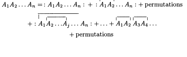 | Moyal product for Wightman propagator ##\Delta_H## ## \begin{aligned} & A_1 \star_H A_2 = \\ & ((-)\cdot (-)) \circ \exp \left( \hbar \int (\Delta_H)^{ab}(x,y) \frac{\delta}{\delta \mathbf{\Phi}^a(x)} \otimes \frac{\delta}{\delta \mathbf{\Phi}^b(y)} \right)(A_1 \otimes A_2) \end{aligned}## | |
| perturbative expansion of 3) via 1) | Feynman diagrams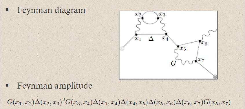 | Moyal product for Feynman propagator ##\Delta_F## ## \begin{aligned} & A_1 \star_F A_2 = \\ & ((-)\cdot (-)) \circ \exp \left( \hbar \int (\Delta_F)^{ab}(x,y) \frac{\delta}{\delta \mathbf{\Phi}^a(x)} \otimes \frac{\delta}{\delta \mathbf{\Phi}^b(y)} \right)(A_1 \otimes A_2) \end{aligned}## |
{#FeynmanDiagramInTwoStages} We now discuss Feynman diagrams and their Feynman amplitudes in two stages: First we consider plain finite multigraphs with linearly ordered vertices but no other labels (def. 15.50 below) and discuss how these generally organize an expansion of the time-ordered products as a sum of distributional products of the given Feynman propagator (prop. 15.51 below). These summands (or their vacuum expectation values) are called the Feynman amplitudes if one thinks of the underlying free field vacuum as having a single “field species” and of the chosen interaction to be a single “interaction vertex”.
But often it is possible and useful to identify different field species and different interaction vertices. In fact, in applications, this choice is typically evident and not highlighted as a choice. We make it explicit below as def. 15.52. Such a choice makes both the interaction term as well as the Feynman propagator decompose as sums (remark 15.53 below). Accordingly then, after “multiplying out” the products of these sums that appear in the Feynman amplitudes, these, too, decompose further as sums indexed by multigraphs whose edges are labeled by field species, and whose vertices are labeled by interactions. These labeled multigraphs are the Feynman diagrams (def. 15.55 below) and the corresponding summands are the Feynman amplitudes proper (prop. 15.56 below).
Definition 15.50. (finite multigraphs)
A finite multigraph is
- a finite set ##V## (“of vertices”);
- a finite set ##E## (“of edges”);
- a function ##E \overset{p}{\to} \left\{ {\,\atop \,} \{v_1, v_2\} = \{v_2, v_1\} \;\vert\; v_1, v_2 \in V \,,\; v_1 \neq v_2 {\, \atop \,} \right\}##(sending any edge to the unordered pair of distinct vertices that it goes between).
A choice of linear order on the set of vertices of a finite multigraph is a choice of bijection of the form
$$
V \simeq \{1, 2, \cdots, \nu\}
\,.
$$
Hence the isomorphism classes of a finite multigraphs with linearly ordered vertices are characterized by
- a natural number$$
\nu := {\vert V\vert} \in \mathbb{N}
$$(the number of vertices); - for each ##i \lt j \in \{1, \cdots, \nu\}## a natural number$$
e_{i,j} := {\vert p^{-1}(\{v_i,v_j\})\vert} \in \mathbb{N}
$$(the number of edges between the ##i##th and the ##j##th vertex).
We write ##\mathcal{G}_\nu## for the set of such isomorphism classes of finite multigraphs with linearly ordered vertices identified with ##\{1, 2, \cdots, \nu\}##; and we write
$$
\mathcal{G} \;:=\; \underset{\nu \in \mathbb{N}}{\sqcup} \mathcal{G}_\nu
$$
for the set of isomorphism classes of finite multigraphs with linearly ordered vertices of any number.
Proposition 15.51. (Feynman amplitudes of finite multigraphs)
Let ##(E_{\text{BV-BRST}}, \mathbf{L}’, \Delta_H )## be a relativistic free vacuum according to def. 15.1.
For ##\nu \in \mathbb{N}##, the ##\nu##-fold time-ordered product away from coinciding interaction points, given by prop. 15.42
$$
T_\nu
\;\colon\;
\left(
{\, \atop \,}
LocObs(E_{\text{BV-BRST}})[ [\hbar, g, j] ]
{\, \atop \,}
\right)^{\otimes^\nu_{\mathbb{C}[ [\hbar, g, j] ]}}_{pds}
\longrightarrow
PolyObs(E_{\text{BV-BRST}})_{reg}((\hbar))[ [g , j] ]
$$
is equal to the following formal power series labeled by isomorphism classes of finite multigraphs with ##\nu## linearly ordered vertices, ##\Gamma \in \mathcal{G}_\nu## (def. 15.50):
| $$ \label{FeynmanAmplitudeExpansionOfTimeOrderedProductAwayFromDiagonal} \begin{aligned} & T_\nu(O_1, \cdots , O_\nu) \\ & = \underset{\Gamma \in \mathcal{G}_\nu}{\sum} \Gamma\left(O_i)_{i = 1}^\nu\right) \\ & := \underset{ \Gamma \in \mathcal{G}_\nu }{\sum} prod \circ \underset{ r \lt s \in \{1, \cdots, \nu\} }{\prod} \frac{\hbar^{e_{r,s}}}{e_{r,s}!} \left\langle (\Delta_{F})^{e_{r,s}} , \frac{\delta^{e_{r,s}}}{\delta \mathbf{\Phi}_r^{e_{r,s}}} \frac{\delta^{e_{r,s}}}{\delta \mathbf{\Phi}_s^{e_{r,s}}} \right\rangle \left( O_1 \otimes \cdots \otimes O_{\nu} \right) \\ & := \underset{ \Gamma \in \mathcal{G}_\nu }{\sum} ((-) \cdot \cdots \cdot (-)) \circ \underset{ r \lt s \in \{1, \cdots,\nu\} }{\prod} \frac{\hbar^{e_{r,s}}}{e_{r,s}!} \\ & \phantom{AAA} \underset{i = 1, \cdots e_{r,s}}{\prod} \underset{\Sigma \times \Sigma}{\int} dvol_\Sigma(x_i) dvol_\Sigma(y_i) \, \Delta_F^{a_i b_i}(x_i,y_i) \\ & \phantom{AAAAAA} \left( O_1 \otimes \cdots \otimes O_{r-1} \otimes \frac{ \delta^{e_{r,s}} O_r }{ \delta \mathbf{\Phi}^{a_1}(x_1) \cdots \delta \mathbf{\Phi}^{a_{e_{r,s}}}(x_{e_{r,s}}) } \otimes O_{r+1} \otimes \cdots \otimes O_{s-1} \otimes \frac{ \delta^{e_{r,s}} O_s }{ \delta \mathbf{\Phi}^{b_1}(y_1) \cdots \delta \mathbf{\Phi}^{b_{e_{r,s}}}(y_{e_{r,s}}) } \otimes O_{s+1} \otimes \cdots \otimes O_\nu \right) \,, \end{aligned} $$ | (241) |
where ##e_{r,s} := e_{r,s}(\Gamma)## is, for short, the number of edges between vertex ##r## and vertex ##s## in the finite multigraph ##\Gamma## of the outer sum, according to def. 15.50.
Here the summands of the expansion (241)
| $$ \label{FeynmanAmplitude} \Gamma\left( (O_i)_{i = 1}^\nu\right) \;:=\; prod \circ \underset{ r \lt s \in \{1, \cdots,\nu\} }{\prod} \frac{\hbar^{e_{r,s}}}{e_{r,s}!} \left\langle (\Delta_{F})^{e_{r,s}} , \frac{\delta^{e_{r,s}}}{\delta \mathbf{\Phi}_r^{e_{r,s}}} \frac{\delta^{e_{r,s}}}{\delta \mathbf{\Phi}_s^{e_{r,s}}} \right\rangle \left( O_1 \otimes \cdots \otimes O_{\nu} \right) \;\in\; PolyObs(E_{\text{BV-BRT}})((\hbar))[ [g,j ] ] $$ | (242) |
and/or their vacuum expectation values
$$
\left\langle
\Gamma\left((V_i)_{i = 1}^v\right)
\right\rangle
\;\in\;
\mathbb{C}((\hbar))[ [ h, j] ]
$$
are called the Feynman amplitudes for scattering processes in the given free field vacuum of shape ##\Gamma## with interaction vertices ##O_i##. Their expression as products of distributions via algebraic expression on the right-hand side of (242) is also called the Feynman rules.
(Keller 10, IV.1)
Proof. We proceed by induction over the number ##v## of vertices. The statement is trivially true for a single vertex. So assume that it is true for ##v \geq 1## vertices. It follows that
$$
\begin{aligned}
& T(O_1, \cdots, O_\nu, O_{\nu+1})
\\
& =
T( T(O_1, \cdots ,O_\nu), O_{\nu+1} )
\\
&=
prod
\circ
\exp\left(
\left\langle
\hbar \Delta_F,
\frac{\delta}{\delta \mathbf{\Phi}}
\otimes
\frac{\delta}{\delta \mathbf{\Phi}}
\right\rangle
\right)
\left(
\left(
prod
\circ
\!\!\!\!
\underset{\Gamma \in \mathcal{G}_\nu }{\sum}
\underset{ { r \lt s } \atop { \in \{1, \cdots, \nu\} } }{\prod}
\frac{1}{e_{r,s}!}
\left\langle
(\hbar \Delta_F)^{e_{r,s}}
\,,\,
\frac{\delta^{e_{r,s}}}{\delta \mathbf{\Phi}_r^{e_{r,s}}}
\frac{\delta^{e_{r,s}}}{ \delta \mathbf{\Phi}_s^{e_{r,s}} }
\right\rangle
(O_1 \otimes \cdots \otimes O_\nu)
\right)
\,\otimes\,
O_{\nu+1}
\right)
\\
& =
prod
\circ
\underset{\Gamma \in \mathcal{G}_\nu }{\sum}
\\
& \phantom{=}
\underset{ { r \lt s } \atop { \in \{1,\cdots, \nu\}} }{\prod}
\frac{1}{e_{r,s}!}
\left\langle
(\hbar \Delta_F)^{e_{r,s}}
\,,\,
\frac{\delta^{e_{r,s}}}{\delta \mathbf{\Phi}_r^{e_{r,s}}}
\frac{\delta^{e_{r,s}}}{ \delta \mathbf{\Phi}_s^{e_{r,s}} }
\right\rangle
\\
& \phantom{=}
\underset{
{ e_{\nu+1} =}
\atop
{ e_{1,{\nu+1}} + \cdots + e_{\nu,\nu + 1} }
}{\sum}
\underset{
= (e_{1,\nu + 1}) \cdots (e_{\nu,\nu+1}))
}{
\underbrace{
\frac{
\left(
{ e_{\nu + 1} }
\atop
{ (e_{1, \nu + 1}), \cdots, (e_{\nu , \nu+1}) }
\right)
}{
( e_{\nu+1} ) !
}
}
}
\left\langle
(\hbar \Delta_F)^{e_{\nu+1}}
\left(
\frac{\delta^{e_{1,\nu+1}} O_1 }{\delta \mathbf{\Phi}^{e_{1,\nu+1}}}
\otimes
\cdots
\otimes
\frac{
\delta^{e_{\nu,\nu+1}} O_\nu
}{
\delta \mathbf{\Phi}^{e_{\nu,\nu+1}}
}
\;\otimes\;
\frac{
\delta^{ e_{\nu + 1} } O_{\nu+1}
}{
\delta \mathbf{\Phi}^{e_{1,\nu+1} + \cdots + e_{\nu,\nu+1}}
}
\right\rangle
\right)
\\
&=
prod
\circ
\underset{\Gamma \in \mathcal{G}_{\nu+1} }{\sum}
\underset{ { r \lt s } \atop { \in \{1, \cdots, \nu+1\} } }{\prod}
\tfrac{1}{e_{r,s}!}
\left\langle
(\hbar \Delta_F)^{e_{r,s}}
\,,\,
\frac{\delta^{e_{r,s}}}{\delta \mathbf{\Phi}_r^{e_{r,s}}}
\frac{\delta^{e_{r,s}}}{\delta \mathbf{\Phi}_s^{e_{r,s}}}
\right\rangle
(O_1 \otimes \cdots \otimes O_{\nu+1})
\end{aligned}
$$
The combinatorial factor over the brace is the multinomial coefficient expressing the number of ways of distributing ##e_{\nu+1}##-many functional derivatives to ##v## factors, via the product rule, and quotient by the factorial that comes from the exponential in the definition of the star product.
Here in the first step, we used the associativity (237) of the restricted time-ordered product, in the second step we used the induction assumption, in the third we passed the outer functional derivatives through the pointwise product using the product rule, and in the fourth step, we recognized that this amounts to summing in addition over all possible choices of sets of edges from the first ##v## vertices to the new ##\nu+1##st vertex, which yields in total the sum over all diagrams with ##\nu+1## vertices.
If the free field theory is decomposed as a direct sum of free field theories (def. 15.52 below), we obtain a more fine-grained concept of Feynman amplitudes, associated not just with a finite multigraph, but also with the labeling of this graph by field species and interaction types. These labeled multigraphs are the genuine Feynman diagrams (def. 15.55 below):
Definition 15.52. (field species and interaction vertices)
Let ##(E_{\text{BV-BRST}}, \mathbf{L}’, \Delta_H )## be a relativistic free vacuum according to def. 15.1, and let ##g S_{int} + j A \;\in\; LocObs(E_{\text{BV-BRST}})[ [ \hbar , g , j] ]\langle g,j \rangle## be a local observable regarded as an adiabatically switched interaction action functional.
Then
- a choice of field species is a choice of decomposition of the BV-BRST field bundle ##E_{\text{BV-BRST}}## as a fiber product over finite set ##Spec = \{sp_1, sp_2, \cdots, sp_n\}## of (graded super-) field bundles$$
E_{\text{BV-BRST}}
\;\simeq\;
E_{sp_1} \times_{\Sigma} \cdots \times_\Sigma E_{sp_n}
\,,
$$such that the gauge fixed free Lagrangian density ##\mathbf{L}’## is the sum$$
\mathbf{L}’ \;=\; \mathbf{L}’_{sp_1} + \cdots + \mathbf{L}’_{sp_n}
$$of free Lagrangian densities$$
\mathbf{L}’_{sp_i} \in \Omega^{p+1,0}_\Sigma(E_i)
$$on these separate field bundles. - a choice of interaction vertices and external vertices is a choice of sum decomposition$$
g S_{int} + j A
\;=\;
\underset{i \in Ext}{\sum} g S_{int,i}
+
\underset{j \in Int}{\sum} j A_j
$$parameterized by finite sets ##Int## and ##Ext##, to be called the sets of internal vertex labels and external vertex labels, respectively.
Remark 15.53. (Feynman propagator for separate field species)
Let ##(E_{\text{BV-BRST}}, \mathbf{L}’, \Delta_H )## be a relativistic free vacuum according to def. 15.1.
Then a choice of field species as in def. 15.52
induces a corresponding decomposition of the Feynman propagator of the gauge fixed free field theory
$$
\Delta_F
\;\in\;
\Gamma’_{\Sigma \times \Sigma}( E_{\text{BV-BRST}} \boxtimes E_{\text{BV-BRST}} )
$$
as the sum of Feynman propagators for each of the chosen field species:
$$
\Delta_F
\;=\;
\Delta_{F,1} + \cdots + \Delta_{F,n}
\;\in\;
\underset{i = 1}{\overset{n}{\oplus}}
\Gamma’_{\Sigma \times \Sigma}( E_{sp_i} \boxtimes E_{sp_i} )
\;\subset\;
\Gamma’_{\Sigma \times \Sigma}( E_{\text{BV-BRST}} \boxtimes E_{\text{BV-BRST}} )
$$
hence in components, with ##(\phi^A## the collective field coordinates on ##E_{\text{BV-BRST}}##, this decomposition is of the form
$$
\left(
\Delta_F^{A, B}
\right)
\;=\;
\left(
\array{
(\Delta_{F,1}^{a b}) & 0 & 0 & \cdots & 0
\\
0 & (\Delta_{F,2}^{\alpha \beta}) & 0 & \cdots & 0
\\
\vdots & & & & \vdots
\\
0 & \cdots & \cdots & 0 & (\Delta_{F,n}^{i j})
}
\right)
$$
Example 15.54. (field species in quantum electrodynamics)
The field bundle for Lorenz gauge fixed quantum electrodynamics on Minkowski spacetime ##\Sigma## admits a decomposition into field species, according to def. 15.52, as
$$
E_{\text{BV-BRST}}
\;=\;
\underset{
\text{Dirac}
\atop
\text{field}
}{
\underbrace{
(S_{odd} \times \Sigma)
}}
\times_\Sigma
\underset{
{\text{electromagnetic field &}}
\atop
{\text{Nakanishi-Lautrup field}}
}{
\underbrace{
T^\ast\Sigma
\times_\Sigma
(\mathbb{R} \times \Sigma)
}}
\times_\Sigma
\underset{
\text{ghost field}
}{
\underbrace{
(\mathbb{R}[1] \times \Sigma)
}
}
\times_\Sigma
\underset{
\text{antighost field}
}{
\underbrace{
(\mathbb{R}[-1] \times \Sigma)
}
}
$$
(by example 5.11) and example 12.8)).
The corresponding sum decomposition of the Feynman propagator, according to remark 15.53, is
$$
\Delta_F
\;=\;
\underset{
\text{Dirac}
\atop
\text{field}
}{
\underbrace{
\Delta_F^{\text{electron}}
}
}
+
\underset{
\text{electromagnetic field &}
\atop
\text{Nakanishi-Lautrup field}
}{
\underbrace{
\left(
\array{
\Delta_F^{photon} & *
\\
* & *
}
\right)
}
}
+
\Delta_F^{ghost}
+
\Delta_F^{\text{antighost}}
\,,
$$
where
- ##\Delta_F^{\text{electron}}## is the electron propagator (def. link ));
- ##\Delta_F^{photon}## is the photon propagator in Gaussian-averaged Lorenz gauge (prop. 12.9);
- the ghost field and antighost field Feynman propagators ##\Delta_F^{ghost}##, and ##\Delta_F^{antighost}## are each one copy of the Feynman propagator of the real scalar field (prop. 9.64), while the Nakanishi-Lautrup field contributes a mixing with the photon propagator, notationally suppressed behind the star-symbols above.
Definition 15.55. (Feynman diagrams)
Let ##(E_{\text{BV-BRST}}, \mathbf{L}’, \Delta_H )## be a relativistic free vacuum according to def. 15.1, and let ##g S_{int} + j A \;\in\; LocObs(E_{\text{BV-BRST}})[ [ \hbar , g , j] ]\langle g,j \rangle## be a local observable regarded as an adiabatically switched interaction action functional.
Let moreover
$$
E_{\text{BV-BRST}}
\;\simeq\;
\underset{sp \in Spec}{\times} E_{sp}
\,,
$$
be a choice of field species, according to def 15.52,
$$
g S_{int} + j A
\;=\;
\underset{i \in Ext}{\sum} g S_{int,i}
+
\underset{j \in Int}{\sum} j A_j
$$
a choice of internal and external interaction vertices according to def. 15.52.
With these choices, we say that a Feynman diagram ##(\Gamma, vertlab, edgelab)## is
- a finite multigraph with linearly ordered vertices (def. 15.50)$$
\Gamma \in \mathcal{G}
\,,
$$ - a function from its vertices$$
vertlab \;\colon\; V_{\Gamma} \longrightarrow Int \sqcup Ext
$$to the disjoint union of the chosen sets of internal and external vertex labels; - a function from its edges$$
edgelab \;\colon\; E_{\Gamma} \to Spec
$$to the chosen set of field species.
We write
$$
\array{
\mathcal{G}^{Feyn}
&\overset{\text{forget} \atop \text{labels}}{\longrightarrow}&
\mathcal{G}
\\
(\Gamma,vertlab, edgelab) &\mapsto& \Gamma
}
$$
for the set of isomorphism classes of Feynman diagrams with labels in ##Sp##, refining the set of isomorphisms of plain finite multigraphs with linearly ordered vertices from def. 15.50.
Proposition 15.56. (Feynman amplitudes for Feynman diagrams)
Let ##(E_{\text{BV-BRST}}, \mathbf{L}’, \Delta_H )## be a relativistic free vacuum according to def. 15.1, and let ##g S_{int} + j A \;\in\; LocObs(E_{\text{BV-BRST}})[ [ \hbar , g , j] ]\langle g,j \rangle## be a local observable regarded as an adiabatically switched interaction action functional.
Let moreover
$$
E_{\text{BV-BRST}}
\;\simeq\;
\underset{sp \in Spec}{\times} E_{sp}
\,,
$$
be a choice of field species, according to def 15.52, hence inducing, by remark 15.53, a sum decomposition of the Feynman propagator
| $$ \label{FeynmanPropagatorSumOverFieldSpecies} \Delta_F \;=\; \underset{sp \in Spec}{\sum}\Delta_{F,sp} \,, $$ | (243) |
and let
| $$ \label{VertexDecompositionFeynmanAmplitude} g S_{int} + j A \;=\; \underset{i \in Ext}{\sum} g S_{int,i} + \underset{j \in Int}{\Sum} j A_j $$ | (244) |
be a choice of internal and external interaction vertices according to def. 15.52.
Then by “multiplying out” the products of the sums (243) and (244) in the formula (242) for the Feynman amplitude ##\Gamma\left( (g S_{int} + j A))_{i = 1}^\nu \right)## (def. 15.51) this decomposes as a sum of the form
$$
\Gamma\left(
(g S_{int} + j A)_{i = 1}^\nu
\right)
\;=\;
\underset{
{ V_\Gamma \overset{vertlab}{\longrightarrow} Int \sqcup Ext}
\atop
{ E_\Gamma \overset{edgelab}{\longrightarrow} Spec }
}{\sum}
\left(
\Gamma,
edgelab, vertlab
\right)
(g S_{int} + j A)
$$
overall ways of labeling the vertices ##v## of ##\Gamma## by the internal or external vertex labels, and the edges ##e## of ##\Gamma## by field species. The corresponding summands
$$
\left(
\Gamma,
edgelab,
vertlab
\right)
(g S_{int} + j A)
\;\in\;
PolyObs(E_{\text{BV-BRST}})[ [ \hbar, g, j] ]
$$
or rather their vacuum expectation value
$$
\left\langle
\left(
\Gamma,
edgelab, vertlab
\right)
(g S_{int} + j A)
\right\rangle
\;\in\;
\mathbb{C}[ [ \hbar, g, j ] ]
$$
are called the _Feynman amplitude associated with these Feynman diagrams.
Example 15.57. (Feynman amplitudes in causal perturbation theory — an example of QED)
To recall, in perturbative quantum field theory, Feynman diagrams (def. 15.55) are labeled finite multigraphs (def. 15.50) that encode products of Feynman propagators, called Feynman amplitudes (prop. 15.51) which in turn contribute to probability amplitudes for physical scattering processes — scattering amplitudes (example 15.12):
The Feynman amplitudes are the summands in the Feynman perturbation series-expansion (example 15.58) of the scattering matrix (def. 15.3)
$$
\mathcal{S}
\left(
S_{int}
\right)
=
\underset{k \in \mathbb{N}}{\sum}
\frac{1}{k!}
\frac{1}{(i \hbar)^k}
T( \underset{k \, \text{factors}}{\underbrace{S_{int}, \cdots , S_{int}}} )
$$
of a given interaction Lagrangian density ##L_{int}## (def. 5.1).
The Feynman amplitudes are the summands in an expansion of the time-ordered products ##T(\cdots)## (def. 15.31) of the interaction with itself, which, away from coincident vertices, is given by the star product of the Feynman propagator ##\Delta_F## (prop. 15.42), via the exponential contraction
$$
T(S_{int}, S_{int})
\;=\;
prod \circ \exp
\left(
\hbar
\int \Delta_{F}^{a b}(x,y)
\frac{\delta}{\delta \mathbf{\Phi}^a(x)}
\otimes
\frac{\delta}{\delta \mathbf{\Phi}(y)}
\right)
( S_{int} \otimes S_{int} )
\,.
$$
Each edge in a Feynman diagram corresponds to a factor of a Feynman propagator in ##T( \underset{k \, \text{factors}}{\underbrace{S_{int} \cdots S_{int}}} )##, being a distribution of two variables; and each vertex corresponds to a factor of the interaction Lagrangian density at ##x_i##.
For example, quantum electrodynamics (example 5.11) in Gaussian-averaged Lorenz gauge (example 12.8) involves (via example 15.54):
- the Dirac field modeling the electron, with Feynman propagator called the electron propagator (def. 9.72), here to be denoted$$
\Delta \phantom{AAAA} \text{electron propagator}
$$ - the electromagnetic field modeling the photon, with Feynman propagator called the photon propagator (prop. 12.9), here to be denoted$$
G \phantom{AAAA} \text{photon propagator}
$$ - the electron-photon interaction (47)$$
L_{int}
\;=\;
\underset{
\text{interaction}
}{
\underbrace{
i g
(\gamma^\mu)^\alpha{}_\beta
}
}
\,
\underset{
{ \text{incoming} \atop \text{electron} }
\atop
\text{field}
}{\underbrace{\overline{\psi_\alpha}}}
\;
\underset{
{
\,
\atop
\text{photon}
}
\atop
\text{field}
}{\underbrace{a_\mu}}
\;
\underset{
{\text{outgoing} \atop \text{electron} }
\atop
\text{field}
}{\underbrace{\psi^\beta}}
$$
The Feynman diagram for the electron-photon interaction alone is
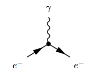
where the solid lines correspond to the electron and the wiggly line to the photon. The corresponding product of distributions (prop. 9.34) is (written in generalized function-notation, example 9.10)
$$
\underset{
\text{loop order}
}{
\underbrace{
\hbar^{3/2-1}
}
}
\underset{
\text{electron-photon}
\atop
\text{interaction}
}{
\underbrace{
i g (\gamma^\mu)^\alpha{}_\beta
}
}
\,.
\,
\underset{
{\text{incoming} \atop \text{electron}}
\atop
\text{propagator}
}{
\underbrace{
\overline{\Delta(-,x)}_{-, \alpha}
}
}
\underset{
{
\,
\atop
\text{photon}
}
\atop
\text{propagator}
}{
\underbrace{
G(x,-)_{\mu,-}
}
}
\underset{
{ \text{outgoing} \atop \text{electron} }
\atop
\text{propagator}
}{
\underbrace{
\Delta(x,-)^{\beta, -}
}
}
$$
Hence a typical Feynman diagram in the QED Feynman perturbation series induced by this electron-photon interaction looks as follows:
where on the bottom the corresponding Feynman amplitude product of distributions is shown; now notationally suppressing the contraction of the internal indices and all prefactors.
For instance the two solid edges between the vertices ##x_2## and ##x_3## correspond to the two factors of ##\Delta(x_2,x_2)##:
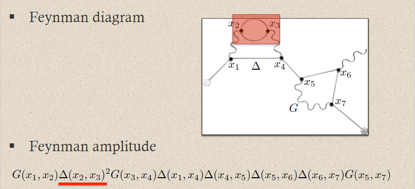
This way each sub-graph encodes its corresponding subset of factors in the Feynman amplitude:
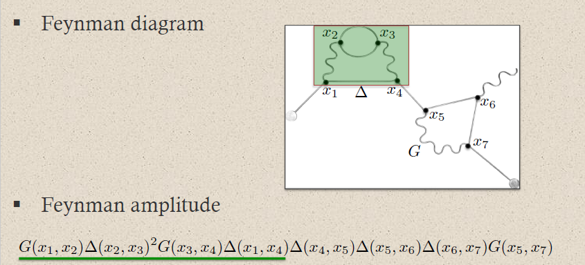
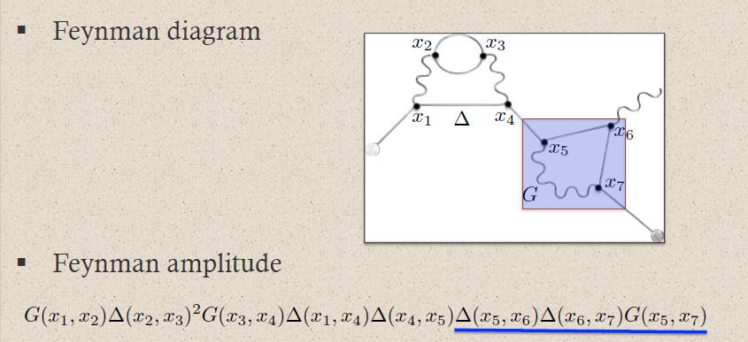
graphics grabbed from Brouder 10
A priori this product of distributions is defined away from coincident vertices: ##x_i \neq x_j## (prop. 15.42 below). The definition at coincident vertices ##x_i = x_j## requires a choice of extension of distributions (def. 16.10 below) to the diagonal locus of coincident interaction points. This choice is the (“re-“)normalization (def. 15.46 below) of the Feynman amplitude.
Example 15.58. (Feynman perturbation series)
Let ##(E_{\text{BV-BRST}}, \mathbf{L}’, \Delta_H )## be a relativistic free vacuum according to def. 15.1, and let
$$
g S_{int} + j A
\;\in\;
LocObs(E_{\text{BV-BRST}})[ [ \hbar, g, h ] ]\langle g , j\rangle
$$
be a local observable, regarded as an adiabatically switched interaction action functional.
By prop. 15.51 every choice of perturbative S-matrix (def. 15.3)
$$
\mathcal{S}(g S_{int} + j A)
\;\in\;
PolyObs(E_{\text{BV-BRST}})_{mc}((\hbar))[ [ g, j ] ] +
$$
has an expansion as a formal power series of the form
$$
\mathcal{S}(g S_{int} + j A)
\;=\;
\underset{\Gamma \in \mathcal{G}}{\sum}
\Gamma\left( (g S_{int} + j A)_{i = 1}^{\nu(\Gamma)}\right)
\,,
$$
where the series is overall finite multigraphs with linearly ordered vertices ##\Gamma## (def. 15.50), and the summands are the corresponding (“re”-)normalized (def. 15.46) Feynman amplitudes (prop. 15.51).
If moreover a choice of field species and of internal and external interaction vertices is made, according to def. 15.52, then this series expansion refines to an expansion over all Feynman diagrams ##(\Gamma,edgelab, vertlab)## (def. 15.55) of Feynman amplitudes ##(\Gamma, edgelab,vertlab)(g S_{int} + j A)## (def. 15.56):
$$
\mathcal{S}(g S_{int} + j A)
\;=\;
\underset{(\Gamma,edgelab, vertlab) \in \mathcal{G}^{Feyn}}{\sum}
(\Gamma, edgelab,vertlab)(g S_{int} + j A)
\,,
$$
Expressed in this form the S-matrix is known as the Feynman perturbation series.
Remark 15.59. (no tadpole Feynman diagrams)
In the definition of finite multigraphs in def. 15.50 there are no edges considered that go from any vertex to itself. Accordingly, there are no such labeled edges in Feynman diagrams (def. 15.55):

In pQFT these diagrams are called tadpoles, and their non-appearance is considered part of the Feynman rules (prop. 15.51). Via prop. 15.51 this condition reflects the nature of the star product (def. 13.18) which always contracts different tensor product factors with the Feynman propagator before taking their pointwise product.
Beware that in graph theory these tadpoles are called “loops”, while here in pQFT a “loop” in a planar graph refers instead to what in graph theory is called a face of the graph, see the discussion of loop order in prop. 15.68 below.
(Keller 10, remark II.8 and proof of prop. II.7)
Effective action
We have seen that the Feynman perturbation series expresses the S-matrix as a formal power series of Feynman amplitudes labeled by Feynman diagrams. Now the Feynman amplitude associated with a disjoint union of connected Feynman diagrams (def. 15.60 below) is just the product of the amplitudes of the connected components (prop. 15.64 below). This allows re-organizing the Feynman perturbation series as the ordinary exponential of the Feynman perturbation series restricted to just connected Feynman diagrams. The latter is called the effective action (def. 15.62 below) because it allows expressing vacuum expectation values of the S-matrix as an ordinary exponential (equation (246) below).
Definition 15.60. (connected graphs)
Given two finite multigraphs ##\Gamma_1, \Gamma_2 \in \mathcal{G}## (def. 15.50), their disjoint union
$$
\Gamma_1 \sqcup \Gamma_2
\;\in\;
\mathcal{G}
$$
is the finite multigraph whose set of vertices and set of edges are the disjoint unions of the corresponding sets of ##\Gamma_1## and ##\Gamma_2##
$$
V_{\Gamma_1 \sqcup \Gamma_2}
\;:=\;
V_{\Gamma_1} \sqcup V_{\Gamma_2}
$$
$$
E_{\Gamma_1 \sqcup \Gamma_2}
\;:=\;
E_{\Gamma_1} \sqcup E_{\Gamma_2}
$$
and whose vertex-assigning function ##p## is the corresponding function on disjoint unions
$$
p_{\Gamma_1 \sqcup \Gamma_2}
\;:=\;
p_{\Gamma_1} \sqcup p_{\Gamma_2}
\,.
$$
The operation induces a pairing on the set ##\mathcal{G}## of isomorphism classes of finite multigraphs
$$
(-) \sqcup (-)
\;\colon\;
\mathcal{G} \times \mathcal{G}
\longrightarrow
\mathcal{G}
\,.
$$
A finite multigraph ##\Gamma \in \mathcal{G}## (def. 15.50) is called connected if it is not the disjoint union of two non-empty finite multigraphs.
We write
$$
\mathcal{G}_{conn}
\subset
\mathcal{G}
$$
for the subset of isomorphism classes of connected finite multigraphs.
Lemma 15.61. (Feynman amplitudes multiply under the disjoint union of graphs)
Let
$$
\Gamma
\;=\;
\Gamma_1
\sqcup
\Gamma_2
\sqcup
\cdots
\sqcup
\Gamma_n
\;\in\; \mathcal{G}
$$
be disjoint union of graphs (def. 15.60). then corresponding Feynman amplitudes (prop. 15.51) multiply by the pointwise product (def. 7.1):
$$
\Gamma\left( g S_{int} + j A)_{i = 1}^{\nu(\Gamma)} \right)
\;=\;
\Gamma_1\left( (g S_{int} + j A)_{i = 1}^{\nu(\Gamma_1)}\right)
\cdot
\Gamma_2\left( (g S_{int} + j A)_{i = 1}^{\nu(\Gamma_2)} \right)
\cdot
\cdots
\cdot
\Gamma_n\left( (g S_{int} + j A)_{i = 1}^{\nu(\Gamma_n)} \right)
\,.
$$
Proof. By prop. 15.42 the contributions to the S-matrix away from coinciding interaction points are given by the star product induced by the Feynman propagator, and specifically, by prop. 15.51, the Feynman amplitudes are given this way. Moreover, the star product (def. 13.18) is given by first contracting with powers of the Feynman propagator and then multiplying all resulting terms with the pointwise product of observables. This implies the claim by the nature of the combinatorial factor in the definition of the Feynman amplitudes (prop. 15.51).
Definition 15.62. (effective action)
Let ##(E_{\text{BV-BRST}}, \mathbf{L}’, \Delta_H )## be a relativistic free vacuum according to def. 15.1, let ##\mathcal{S}## be an S-matrix scheme for perturbative QFT around this vacuum (def. 15.3) and let
$$
g S_{int} + j A
\;\in\;
LocObs(E_{\text{BV-BRST}})[ [ \hbar, g, h ] ]
$$
be a local observable.
Recall that for each finite multigraph ##\Gamma \in \mathcal{G}## (def. 15.50) the Feynman perturbation series for ##\mathcal{S}(g S_{int} + j A)## (example 15.58)
$$
\mathcal{S}(g S_{int} + j A)
\;=\;
\underset{\Gamma \in \mathcal{G}}{\sum}
\Gamma\left( (g S_{int} + j A)_{i = 1}^{v(\Gamma)} \right)
$$
contributes with a (“re”-)nromalized Feynman amplitude ##\Gamma\left( (g S_{int} + j A)_{i = 1}^v\right) \in PolyObs(E_{\text{BV-BRST}})((\hbar))[ [ g, j ] ]##.
We say that the corresponding effective action is ##i \hbar## times the sub-series
| $$ \label{ExpansionEffectiveAction} S_{eff}(g,j) \;:=\; i \hbar \underset{\Gamma \in \mathcal{G}_{conn}}{\sum} \Gamma\left( (g S_{int} + j A)_{i = 1}^{\nu(\Gamma)} \right) \;\in\; PolyObs(E_{\text{BV-BRST}})((\hbar))[ [ g, j ] ] $$ | (245) |
of Feynman amplitudes that are labeled only by the connected graphs ##\Gamma \in \mathcal{G}_{conn} \subset \mathcal{G}## (def. 15.60).
(A priori ##S_{eff}(g,j)## could contain negative powers of ##\hbar##, but it turns out that it does not; this is prop. 15.68 below.)
Remark 15.63. (terminology for “effective action”)
Beware differing conventions of terminology:
- In the perspective of effective quantum field theory (remark 16.27 below), the effective action in def. 15.62 is sometimes called the effective potential at scale ##\Lambda = 0## (see prop. 15.62 below).This terminology originates in restriction to the special example of the scalar field (example 3.5), where the non-derivative Phi^n interactions ##g S_{int} = \underset{n}{\sum} \underset{\Sigma}{\int} g_{sw}^{(n)}(x) (\mathbf{\Phi}(x))^n \, dvol_\Sigma(x)## (example 5.5) are naturally thought of as potential energy-terms.From this perspective the effective action in def. 15.62 is a special case of relative effective actions ##S_{eff,\Lambda}## (“relative effective potentials”, in the case of Phi^n interactions) relative to an arbitrary UV cutoff-scales ##\Lambda## (def. 16.26 below).
- For the special case that$$
j A
:=
\underset{\Sigma}{\int} j_{sw,a}(x) \mathbf{\Phi}^a(x)\, dvol_{\Sigma}(x)
$$ is a regular linear observable (def. 7.30) the effective action according to def. 15.62 is often denoted ##W(j)## or ##E(j)##, and then its functional Legendre transform (if that makes sense) is instead called the effective action, instead.This is because the latter encodes the equations of motion for the vacuum expectation values ##\langle \mathbf{\Phi}(x)_int\rangle## of the interacting field observables; see example 15.66 below.
Notice the different meaning of “effective” in both cases: In the first case, it refers to what is effectively seen of the full pQFT at some UV-cutoff scale, while in the second case it refers to what is effectively seen when restricting attention only to the vacuum expectation values of regular linear observables.
Proposition 15.64. (effective action is logarithm of S-matrix)
Let ##(E_{\text{BV-BRST}}, \mathbf{L}’, \Delta_H )## be a relativistic free vacuum according to def. 15.1, let ##\mathcal{S}## be an S-matrix scheme for perturbative QFT around this vacuum (def. 15.3) and let
$$
g S_{int} + j A
\;\in\;
LocObs(E_{\text{BV-BRST}})[ [ \hbar, g, h ] ]
$$
be a local observable and let
$$
S_{eff}(g,j) \;\in\; PolyObs(E_{\text{BV-BRST}})((\hbar))[ [ g, j] ]
$$
be the corresponding effective action (def. 15.62).
Then then S-matrix for ##g S_{int} + j A## is the exponential of the effective action with respect to the pointwise product ##(-)\cdot (-)## of observables (def. 7.1):
$$
\begin{aligned}
\mathcal{S}(g S_{int} + j A)
& =
\exp_\cdot\left( \tfrac{1}{i \hbar} S_{eff}(g,j) \right)
\\
& :=
1
+
\frac{1}{i \hbar} S_{eff}(g,j)
+
\frac{1}{(i \hbar)^2} S_{eff}(g,j) \cdot S_{eff}(g,j)
+
\frac{1}{(i \hbar)^3} S_{eff}(g,j) \cdot S_{eff}(g,j) \cdot S_{eff}(g,j)
+
\cdots
\end{aligned}
$$
Moreover, this relation passes to the vacuum expectation values:
| $$ \label{ExponentialSeffVEVOfSMatrix} \begin{aligned} \left\langle {\, \atop \,} \mathcal{S}(g S_{int} + j A) {\, \atop \,} \right\rangle & = \left\langle {\, \atop \,} \exp\left( \tfrac{1}{i \hbar} S_{eff}(g,j) \right) {\, \atop \,} \right\rangle \\ & = e^{\tfrac{1}{i \hbar} \langle S_{eff}(g,j) \rangle} \end{aligned} \,. $$ | (246) |
Conversely, the vacuum expectation value of the effective action is to the logarithm of that of the S-matrix:
$$
\left\langle
S_{eff}(g,j)
\right\rangle
\;=\;
i \hbar
\,
\ln
\left\langle
\mathcal{S}(g S_{int} + j A)
\right\rangle
\,.
$$
Proof. By lemma 15.61 the summands in the ##n##th pointwise power of ##\frac{1}{i \hbar}## times the effective action are precisely the Feynman amplitudes ##\Gamma\left((g S_{int} + j A)_{i = 1}^{\nu(\Gamma)}\right)## of finite multigraphs ##\Gamma## with ##n## connected components, where each such appears with multiplicity given by the factorial of ##n##:
$$
\frac{1}{n!}
\left(
\frac{1}{i \hbar}
S_{eff}(g,j)
\right)^n
\;=\;
\underset{
{ \Gamma = \underset{j = 1}{\overset{n}{\sqcup}} \Gamma_j }
\atop
{ \Gamma_j \in \mathcal{G}_{conn} }
}{\sum}
\Gamma\left( (g S_{int} + j A)_{i = 1}^{\nu(\Gamma)} \right)
\,.
$$
It follows that
$$
\begin{aligned}
\exp_\cdot\left(
\frac{1}{i \hbar} S_{int}
\right)
& =
\underset{n \in \mathbb{N}}{\sum}
\underset{
{ \Gamma = \underset{j = 1}{\overset{n}{\sqcup}} \Gamma_j }
\atop
{ \Gamma_j \in \mathcal{G}_{conn} }
}{\sum}
\Gamma\left( (g S_{int} + j A)_{i = 1}^{v(\Gamma)} \right)
\\
& =
\underset{\Gamma \in \mathcal{G}}{\sum}
\Gamma\left( (g S_{int} + j A)_{i = 1}^{v(\Gamma)} \right)
\end{aligned}
$$
yields the Feynman perturbation series by expressing it as a series (re-)organized by a number of connected components of the Feynman diagrams.
To conclude the proof it is now sufficient to observe that taking vacuum expectation values of polynomial observables respects the pointwise product of observables
$$
\left\langle A_1 \cdot A_2 \right\rangle
\;=\;
\left\langle
A_1
\right\rangle
\,
\left\langle
A_2
\right\rangle
\,.
$$
This is because the Hadamard vacuum state ##\langle -\rangle \colon PolyObs(E_{\text{BV-BRST}})[ [ \hbar, g, j] ] \to \mathbb{C}[ [\hbar, g, j ] ]## simply picks the zero-order monomial term, by prop. 14.15), and under multiplication of polynomials the zero-order terms are multiplied.
This immediately implies the following important fact:
Proposition 15.65. (in stable vacuum the effective action is generating function for vacuum expectation values of interacting field observables)
Let ##(E_{\text{BV-BRST}}, \mathbf{L}’, \Delta_H )## be a relativistic free vacuum according to def. 15.1, and let ##g S_{int} + j A \;\in\; LocObs(E_{\text{BV-BRST}})[ [ \hbar , g , j] ]\langle g,j \rangle## be a local observable regarded as an adiabatically switched interaction action functional.
If the given vacuum state is stable (def. 15.10) then the vacuum expectation value ##\langle S_{eff}(g,j)\rangle## of the effective action (def. 15.62) is the generating function for the vacuum expectation value of the interacting field observable ##A_{int}## (def. 15.8) in that
$$
\left\langle
A_{int}
\right\rangle
\;=\;
\frac{d}{d j}
S_{eff}(g,j)\vert_{j = 0}
\,.
$$
Proof. We compute as follows:
$$
\begin{aligned}
\frac{d}{d j}
S_{eff}(g,j)
& =
i \hbar
\frac{d}{d j}
\ln
\left\langle
\mathcal{S}(g S_{int} + j A)
\right\rangle
\vert_{j = 0}
\\
& =
i \hbar
\left\langle
\mathcal{S}(g S_{int})
\right\rangle^{-1}
\frac{d}{d j}
\left\langle
\mathcal{S}(g S_{int} + j A)
\right\rangle
\vert_{j = 0}
\\
& =
\left\langle
\frac{d}{d j}
\underset{ \mathcal{Z}(j A) }{
\underbrace{\mathcal{S}(g S_{int})^{-1}
\mathcal{S}(g S_{int} + j A)
}}
\vert_{j = 0}
\right\rangle
\\
& =
\left\langle
A_{int}
\right\rangle
\,.
\end{aligned}
$$
Here in the first step we used prop 15.64, in the second step we applied the chain rule of differentiation>, in the third step we used the definition of vacuum stability (def. 15.10), and in the fourth step we recognized the definition of the interacting field observables (def. 15.8).
Example 15.66. (equations of motion for vacuum expectation values of interacting field observables)
Consider the effective action (def. 15.62) for the case that
$$
\begin{aligned}
j A
& =
\tau{\Sigma}( j_{sw} \phi)
\\
& =
\underset{\Sigma}{\int}
j_{sw}(x) \mathbf{\Phi}(x)
\, dvol_\Sigma(x)
\end{aligned}
$$
is a regular linear observable (this def.), hence the smearing of a field observable (this def.) by an adiabatic switching of the source field
$$
j_{sw} \;\in\; C^\infty_{cp}(\Sigma) \langle j\rangle
\,.
$$
(Here we are notationally suppressing internal field indices, for convenience.)
In this case, the vacuum expectation value of the corresponding effective action is often denoted
$$
W(j_{sw})
$$
and regarded as a function of the adiabatic switching ##j_{sw}## of the source field.
In this case prop. 15.65 says that if the vacuum state is stable, then ##W## is the generating functional for interacting (def. 15.8) field observables (def. 7.2) in that
| $$ \label{WFunctionalDerivative} \left\langle \mathbf{\Phi}(x)_{int} \right\rangle \;=\; \frac{\delta}{\delta j_{sw}(x)} W(j_{sw} = 0) \,. $$ | (247) |
Assume then that there exists a corresponding functional ##\Gamma(\Phi)## of the field histories ##\Phi \in \Gamma_{\Sigma}(E_{\text{BV-BRST}})## (def. 3.1), which behaves like a functional Legendre transform of ##W## in that it satisfies the functional version of the defining equation of Legendre transforms (first derivatives are inverse functions of each other, see this equation):
$$
\frac{\delta }{\delta \Phi(x)}
\Gamma
\left(
\frac{\delta}{\delta j_{sw}(y)} W
\right)
\;=\;
\delta(x,y) j_{sw}(x)
\,.
$$
By (247) this implies that
$$
\frac{\delta }{\delta \Phi(x)}
\Gamma
\left(
\left\langle \mathbf{\Phi}(x)_{int} \right\rangle \right)
\;=\;
0
\,.
$$
This may be read as a quantum version of the principle of extremal action (prop. 7.38) formulated now not for the field histories ##\Phi(x)##, but for the vacuum expectation values, ##\langle \mathbf{\Phi}(x)_{int}\rangle## of their corresponding interacting quantum field observables.
Beware, (as in remark 15.63) that many texts refer to ##\Gamma(\Phi)## as the effective action, instead of its Legendre transform, the generating functional ##W(j_{sw})##.
The perspective of the effective action gives a transparent picture of the order of quantum effects involved in the S-matrix, this is prop. 15.68 below. In order to state this conveniently, we invoke two basic concepts from graph theory:
Definition 15.67. (planar graphs and trees)
A finite multigraph (def. 15.50) is called a planar graph if it admits an embedding into the plane, hence if it may be “drawn into the plane” without intersections, in an evident way.
A finite multigraph is called a tree if for any two of its vertices there is at most one path of edges connecting them, these are examples of planar graphs. We write
$$
\mathcal{G}_{tree}
\subset
\mathcal{G}
$$
for the subset of isomorphism classes of finite multigraphs with linearly ordered vertices (def. 15.50) on those which are trees.
Proposition 15.68. (loop order and tree-level of Feynman perturbation series)
The effective action (def. 15.62) contains no negative powers of ##\hbar##, hence is indeed a formal power series also in ##\hbar##:
$$
S_{eff}(g,j)
\;\in\;
PolyObs(E_{\text{BV-BRST}})[ [ \hbar, g, j ] ]
\,.
$$
and in particular
$$
\left\langle
S_{eff}(g,j)
\right\rangle
\;\in\;
\mathbb{C}[ [ \hbar, g, j] ]
\,.
$$
Moreover, the contribution to the effective action in the classical limit ##\hbar \to 0## is precisely that of Feynman amplitudes of those finite multigraphs (prop. 15.51) which are trees (def. 15.67); thus called the tree level-contribution:
$$
S_{eff}(g,j)\vert_{\hbar = 0}
\;=\;
i \hbar
\underset{\Gamma \in \mathcal{G}_{conn} \cap \mathcal{G}_{tree}}{\sum}
\Gamma\left( (g S_{int} + j A)_{i = 1}^{\nu(\Gamma)} \right)
\,.
$$
Finally, a finite multigraph ##\Gamma## (def. 15.50) which is planar (def. 15.67) and connected (def. 15.60) contributes to the effective action precisely at order
$$
\hbar^{L(\Gamma)}
\,,
$$
where ##L(\Gamma) \in \mathbb{N}## is the number of faces of ##\Gamma##, here called the number of loops of the diagram; here usually called the loop order of ##\Gamma##.
(Beware the terminology clash with graph theory, see the discussion of tadpoles in remark 15.59.)
Proof. By def. 15.3 the explicit ##\hbar##-dependence of the S-matrix is
$$
\mathcal{S}
\left(
S_{int}
\right)
\;=\;
\underset{k \in \mathbb{N}}{\sum}
\frac{1}{k!}
\frac{1}{(i \hbar)^k}
T( \underset{k \, \text{factors}}{\underbrace{S_{int}, \cdots, S_{int}}} )
$$
and by prop. 15.42 the further ##\hbar##-dependence of the time-ordered product ##T(\cdots)## is
$$
T(S_{int}, S_{int})
\;=\;
prod \circ
\exp\left(
\hbar
\left\langle
\Delta_F,
\frac{\delta}{\delta \mathbf{\Phi}}
\otimes
\frac{\delta}{\delta \mathbf{\Phi}}
\right\rangle
\right)
( S_{int} \otimes S_{int} )
\,,
$$
By the Feynman rules (prop. 15.51) this means that
- each vertex of a Feynman diagram contributes a power ##\hbar^{-1}## to its Feynman amplitude;
- each edge of a Feynman diagram contributes a power ##\hbar^{+1}## to its Feynman amplitude.
If we write
$$
E(\Gamma), V(\Gamma) \;\in\; \mathbb{N}
$$
for the total number of vertices and edges, respectively, in ##\Gamma##, this means that a Feynman amplitude corresponding to some ##\Gamma \in \mathcal{G}## contributes precisely at order
| $$ \label{GeneralFeynmanDiagramhbarContribution} \hbar^{E(\Gamma) – V(\Gamma)} \,. $$ | (248) |
So far this holds for arbitrary ##\Gamma##. If however ##\Gamma## is connected (def. 15.60) and planar (def. 15.67), then Euler’s formula asserts that
| $$ \label{ConnectedPlanarGraphEulerCharacteristic} E(\Gamma) – V(\Gamma) \;=\; L(\Gamma) – 1 \,. $$ | (249) |
Hence ##\hbar^{L(\Gamma)- 1}## is the order of ##\hbar## at which ##\Gamma## contributes to the scattering matrix expressed as the Feynman perturbation series.
But the effective action, by definition (245), has the same contributions of Feynman amplitudes but multiplied by another power of ##\hbar^1##, hence it contributes at order
$$
\hbar^{E(\Gamma) – V(\Gamma) + 1} = \hbar^{L(\Gamma)}
\,.
$$
This proves the second claim on loop order.
The first claim, due to the extra factor of ##\hbar## in the definition of the effective action, is equivalent to saying that the Feynman amplitude of every connected finite multigraph contributes powers in ##\hbar## of order ##\geq -1## and contributes at order ##\hbar^{-1}## precisely if the graph is a tree.
Observe that a connected finite multigraph ##\Gamma## with ##\nu \in \mathbb{N}## vertices (necessarily ##\nu \geq 1##) has at least ##\nu-1## edges and precisely ##\nu – 1## edges if it is a tree.
To see this, consecutively remove edges from ##\Gamma## as long as possible while retaining connectivity. When this process stops, the result must be a connected tree ##\Gamma’##, hence a connected planar graph with ##L(\Gamma’) = 0##. Therefore Euler’s formula (249) implies that that ##E(\Gamma’) = V(\Gamma’) -1##.
This means that the connected multigraph ##\Gamma##, in general, has a Feynman amplitude of the order
$$
\hbar^{E(\Gamma) – V(\Gamma)}
=
\hbar^{ \overset{\geq 0}{\overbrace{E(\Gamma) – E(\Gamma’)}} + \overset{= -1}{\overbrace{E(\Gamma’) – V(\Gamma)}} }
$$
and precisely if it is a tree its Feynman amplitude is of order ##\hbar^{-1}##.
Vacuum diagrams
With the Feynman perturbation series and the effective action in hand, it is now immediate to see that there is a general contribution by vacuum diagrams (def. 15.69 below) in the scattering matrix which, in a stable vacuum state, cancels out against the prefactor ##\mathcal{S}(g S_{int})## in Bogoliubov’s formula for interacting field observables.
Definition 15.69. (vacuum diagrams)
Let ##(E_{\text{BV-BRST}}, \mathbf{L}’, \Delta_H )## be a relativistic free vacuum according to def. 15.1, and let ##g S_{int} + j A \;\in\; LocObs(E_{\text{BV-BRST}})[ [ \hbar , g , j] ]\langle g,j \rangle## be a local observable regarded as an adiabatically switched interaction action functional, and consider a choice of decomposition for field species and interaction vertices according to def. 15.52.
Then a Feynman diagram of all whose vertices are internal vertices (def. 15.55) is called a vacuum diagram.
Write
$$
\mathcal{G}^{Feyn}_{vac}
\subset
\mathcal{G}^{Feyn}
$$
for the subset of isomorphism classes of vacuum diagrams among the set of isomorphism classes of all Feynman diagrams, def. 15.55. Similarly, write
$$
\mathcal{G}^{Feyn}_{conn,vac}
\;:=\;
\mathcal{G}^{Feyn}_{conn}
\cap
\mathcal{G}^{Feyn}_{vac}
\;\subset\;
\mathcal{G}^{Feyn}
$$
for the subset of isomorphism classes of Feynman diagrams which are both vacuum diagrams as well as connected graphs (def. 15.60).
Finally, write
$$
S_{eff,vac}(g)
\;:=\;
\underset{ { (\Gamma,vertlab,edgelab) } \atop { \in \mathcal{G}_{conn,vac} } }{\sum}
(\Gamma,vertlab, edgelab)(g S_{int})
\;\in\;
PolyObs(E_{\text{BV-BRST}})_{mc}[ [ \hbar , g ] ]
$$
for the sub-series of that for the effective action (def. 15.62) given only by those connected diagrams which are also vacuum diagrams.
Example 15.70. (2-vertex vacuum diagram in QED)
The vacuum diagram (def. 15.69) with two electron-photon interaction-vertices in quantum electrodynamics (example 5.11) is:
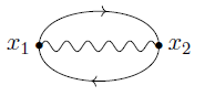
Example 15.71. (vacuum diagram-contribution to S-matrices)
Let ##(E_{\text{BV-BRST}}, \mathbf{L}’, \Delta_H )## be a relativistic free vacuum according to def. 15.1, and let ##g S_{int} + j A \;\in\; LocObs(E_{\text{BV-BRST}})[ [ \hbar , g , j] ]\langle g,j \rangle## be a local observable regarded as an adiabatically switched interaction action functional, and consider a choice of decomposition for field species and interaction vertices according to def. 15.52.
Then the Feynman perturbation series-expansion of the S-matrix (example 15.58) of the interaction-term ##g S_{int}## alone (no source field-contribution) is the series of Feynman amplitudes that are labeled by vacuum diagrams (def. 15.69), hence (by prop. 15.64) the exponential of the vacuum effective action ##S_{eff,vac}## (def. 15.69):
$$
\begin{aligned}
\mathcal{S}(g S_{int})
& =
\exp_\cdot\left( \tfrac{1}{i \hbar} S_{eff,vac}(g,j) \right)
\\
& =
\underset{\Gamma \in \mathcal{G}_{vac}}{\sum}
\Gamma\left(g S_{int}\right)
\end{aligned}
\,.
$$
More generally, the S-matrix with source field-contribution ##j A## included always splits as a pointwise product of the vacuum S_matrix with the Feynman perturbation series overall Feynman graphs with at least one external vertex:
$$
\begin{aligned}
\mathcal{S}(g S_{int} + j A)
\;=\;
\mathcal{S}(g S_{int})
\cdot
\underset{
\text{Feynman perturbation series}
\atop
\text{over diagrams with at least one external vertex}
}{
\underbrace{
\exp_\cdot
\left(
\tfrac{1}{i \hbar} \left( S_{eff}(g,j) – S_{eff,vac}(g) \right)
\right)
}
}
\,,
\end{aligned}
$$
Hence if the free field vacuum state is stable with respect to the interaction ##g S_{int}##, according to def. 15.10, then the vacuum expectation value of a time-ordered product of interacting field observables ##j (A_i)_{int}## (example 15.11) and hence in particular of scattering amplitudes (example 15.12) is given by the Feynman perturbation series (example 15.58) over just the non-vacuum Feynman diagrams, hence over all those diagrams that have at least one external vertex
$$
\begin{aligned}
&
\left(
{\, \atop \,}
supp(A_1)
{\vee\!\!\!\wedge}
supp(A_2)
{\vee\!\!\!\wedge}
\cdots
{\vee\!\!\!\wedge}
supp(A_n)
{\, \atop \,}
\right)
\\
& \Rightarrow
\left\langle
{\, \atop \,}
(A_1)_int
(A_2)_{int}
\cdots
(A_n)_{int}
{\, \atop \,}
\right\rangle
\;=\;
\frac{d^n}{ d j_1 \cdots d j_n}
\left(
\underset{\Gamma \in \mathcal{G} \setminus \mathcal{G}_{vac} }{\sum}
\Gamma(g S_{int} + \sum_i j_i A_i)
\right)_{
\vert j_1, \cdots, j_n = 0
}
\,.
\end{aligned}
$$
This is the way in which the Feynman perturbation series is used in practice for computing scattering amplitudes.
Interacting quantum BV-Differential
So far we have discussed, starting with a BV-BRST gauge fixed free field vacuum, the perturbative construction of interacting field algebras of observables (def. 15.24) and their organization in increasing powers of ##\hbar## and ##g## (loop order, prop. 15.68) via the Feynman perturbation series (example 15.58, example 15.71).
But this interacting field algebra of observables still involves all the auxiliary fields of the BV-BRST gauge fixed free field vacuum (example 15.54), while the actual physical gauge-invariant on-shell observables should be (just) the cochain cohomology of the BV-BRST differential on this enlarged space of observables. Hence for the construction of perturbative QFT to conclude, it remains to pass the BV-BRST differential of the free field Wick algebra of observables to a differential on the interacting field algebra, such that its cochain cohomology is well defined.
Since the time-ordered products away from coinciding interaction points and as well as on regular polynomial observables are uniquely fixed (prop. 15.42), one finds that also this interacting quantum BV-differential is uniquely fixed, on regular polynomial observables, by conjugation with the quantum Møller operators (def. 15.72). The formula that characterizes it there is called the quantum master equation or equivalently the quantum master Ward identity (prop. 15.73 below).
When extending to coinciding interaction points via (“re”-)normalization (def. 15.46) these identities are not guaranteed to hold anymore but maybe imposed as renormalization conditions (def. 15.48, prop. 15.49). Quantum correction to the master Ward identity then implies corrections to Noether’s current conservation laws; this we discuss below.
For the following discussion, recall from the previous chapter how the global BV-differential
$$
\{S’,-\}
\;\colon\;
PolyObs(E_{\text{BV-BRST}})_{reg}[ [\hbar] ]
\longrightarrow
PolyObs(E_{\text{BV-BRST}})_{reg}[ [\hbar] ]
$$
on regular polynomial observables (def. 11.29) as well as the global antibracket ##\{-,-\}## (def. 11.28) are conjugated into the time-ordered product via the time ordering operator ##\mathcal{T} \circ \{-S’,-\} \circ \mathcal{T}^{-}## (def. 14.21, prop. 14.22), which makes
In the same way, we may use the quantum Møller operators to conjugate the BV-differential into the regular part of the interacting field algebra of observables:
Definition 15.72. (interacting quantum BV-differential)
Let ##(E_{\text{BV-BRST}}, \mathbf{L}’, \Delta_H )## be a relativistic free vacuum according to def. 15.1 and let
$$
S_{int}
\;\in\;
PolyObs(E_{\text{BV-BRST}})_{reg}[ [ \hbar, g, j] ]
$$
be a regular polynomial observables, regarded as an adiabatically switched non-point-interaction action functional.
Then the interacting quantum BV-differential on the interacting field algebra on regular polynomial observables (def. 15.45) is the conjugation of the plain global BV-differential ##\{-S’,-\}## (def. 11.28) by the quantum Møller operator induced by ##S_{int}## (def. 15.44):
$$
\mathcal{R} \circ \{-S’, (-)\} \circ \mathcal{R}^{-1}
\;\colon\;
PolyObs(E_{\text{BV-BRST}})_{reg}[ [\hbar] ]
\longrightarrow
PolyObs(E_{\text{BV-BRST}})_{reg}[ [\hbar] ]
\,.
$$
(Rejzner 11, (5.38))
Proposition 15.73. (quantum master equation and quantum master Ward identity on regular polynomial observables)
Consider an adiabatically switched non-point-interaction action functional in the form of a regular polynomial observable in degree 0
$$
S_{int}
\;\in\;
PolyObs(E_{\text{BV-BRST}})_{{reg} \atop {deg = 0}}[ [\hbar] ]
\,,
$$
Then the following are equivalent:
- The quantum master equation (QME)
$$
\label{OnRegularObservablesQuantumMasterEquation}
\tfrac{1}{2} \{ S’ + S_{int}, S’ + S_{int} \}_{\mathcal{T}}
+
i \hbar \Delta_{BV}( S’ + S_{int} )
\;=\;
0
\,.
$$(250) - The perturbative S-matrix (def. 15.43) is ##BV##-closed$$
\{-S’, \mathcal{S}(S_{int})\} = 0
\,.
$$ - The quantum master Ward identity (MWI) on regular polynomial observables in terms of retarded products:
$$
\label{OnRegularObservablesQuantumMasterWardIdentity}
\mathcal{R} \circ \{-S’,(-)\} \circ \mathcal{R}^{-1}
\;=\;
–
\left(
\left\{ S’ + S_{int} \,,\, (-) \right\}_{\mathcal{T}}
+ i \hbar \Delta_{BV}
\right)
$$(251) (Dütsch 18, (4.2))
expressing the interacting quantum BV-differential (def. 15.72) as the sum of the time-ordered antibracket (def. 14.21) with the total action functional ##S’ + S_{int}## and ##i \hbar## times the BV-operator (BV-operator).
- The quantum master Ward identity (MWI) on regular polynomial observables in terms of time-ordered products:
$$
\label{OnRegularObservablesQuantumMasterWardIdentityViaTimeOrdered}
\mathcal{S}(-S_{int})
\star_F
\{-S’, \mathcal{S}(S_{int}) \star_F (-)\}
\;=\;
–
\left(
\left\{ S’ + S_{int} \,,\, (-) \right\}_{\mathcal{T}}
+ i \hbar \Delta_{BV}
\right)
$$(252) (Dütsch 18, (4.8))
(Rejzner 11, (5.35) – (5.38), following Hollands 07, (342)-(345))
Proof. To see that the first two conditions are equivalent, we compute as follows
| $$ \label{QuantumMasterOnRegularObservablesBVDifferentialOfSMatrixInTerms} \begin{aligned} \left\{ -S’, \mathcal{S}(S_{int}) \right\} & = \left\{ -S’ , \exp_{\mathcal{T}} \left( \tfrac{1}{i \hbar} S_{int} \right) \right\} \\ & = \underset{ { \tfrac{-1}{i \hbar} \{S’,S\}_{\mathcal{T}} } \atop { \star_F \exp_{\mathcal{T}} \left( \tfrac{1}{i \hbar} S_{int} \right) } }{ \underbrace{ \left\{ -S’ , \exp_{\mathcal{T}} \left( \tfrac{1}{i \hbar} S_{int} \right) \right\}_{\mathcal{T}} } } – i \hbar \underset{ { \left( \tfrac{1}{i \hbar} \Delta_{BV}(S_{int}) + \tfrac{1}{2 (i \hbar)^2} \left\{ S_{int}, S_{int} \right\}_{\mathcal{T}} \right) } \atop { \star_{F} \exp_{\mathcal{T}} \left( \tfrac{1}{i \hbar} S_{int} \right) } }{ \underbrace{ \Delta_{BV} \left( \exp_{\mathcal{T}} \left( \tfrac{1}{i \hbar} S_{int} \right) \right) } } \\ & = \tfrac{-1}{i \hbar} \underset{ \text{QME} }{ \underbrace{ \left( \{S’,S_{int}\} + \tfrac{1}{2}\{S_{int}, S_{int}\} + i \hbar \Delta_{BV}(S_{int}) \right) } } \star_F \exp_{\mathcal{T}} \left( \tfrac{1}{i \hbar} S_{int} \right) \end{aligned} $$ | (253) |
Here in the first step, we used the definition of the BV-operator (def. 14.23) to rewrite the plain antibracket in terms of the time-ordered antibracket (def. 14.21), then under the second brace we used that the time-ordered antibracket is the failure of the BV-operator to be a derivation (prop. 14.25) and under the first brace the consequence of this statement for application to exponentials (example 14.26). Finally, we collected terms, and to “complete the square” we added the terms on the left of
$$
\frac{1}{2} \underset{= 0}{\underbrace{\{S’, S’\}_{\mathcal{T}}}}
–
i \hbar \underset{ = 0}{\underbrace{ \Delta_{BV}(S’)}} = 0
$$
which vanishes because, by definition of gauge fixing (def. 12.1), the free gauge-fixed action functional ##S’## is independent of antifields.
But since the operation ##(-) \star_F \exp_{\mathcal{T}}\left( \tfrac{1}{i \hbar} S_{int} \right)## has the inverse ##(-) \star_F \exp_{\mathcal{T}}\left( \tfrac{-1}{i \hbar} S_{int} \right)##, this implies the claim.
Next, we show that the quantum master equation implies the quantum master Ward identities.
We use that the BV-differential ##\{-S’,-\}## is a derivation of the Wick algebra product ##\star_H## (lemma link ).
First of all this implies that with ##\{-S’, \mathcal{S}(S_{int})\} = 0## also ##\{-S’, \mathcal{S}(S_{int})^{-1}\} = 0##.
Thus we compute as follows:
$$
\begin{aligned}
\{-S’, -\} \circ \mathcal{R}^{-1}(A)
& =
\{-S’, \mathcal{R}^{-1}(A)\}
\\
& =
\left\{
{ \, \atop \, }
-S’,
\mathcal{S}(S_{int})^{-1}
\star_H
\left( \mathcal{S}(S_{int}) \star_F a \right)
{\, \atop \,}
\right\}
\\
& = \phantom{+}
\underset{
= 0
}{
\underbrace{
\left\{
-S’, \mathcal{S}(S_{int})^{-1}
\right\}
}
}
\star_H
\left(
\mathcal{S}(S_{int}) \star_F A
\right)
\\
& \phantom{=}
+
\mathcal{S}(S_{int})^{-1}
\star_H
\left\{
-S’,
\mathcal{S}(S_{int}) \star_F A
\right\}
\\
& =
\mathcal{S}(S_{int})^{-1}
\star_H
\left(
\underset{
= 1
}{
\underbrace{
\mathcal{S}(+ S_{int})
\star_F
\mathcal{S}(- S_{int})
}
}
\star_F
\left\{
-S’,
\mathcal{S}(S_{int}) \star_F A
\right\}
\right)
\\
& =
\mathcal{S}(S_{int})^{-1}
\star_H
\left(
\mathcal{S}(+ S_{int})
\star_F
\underset{ (\ast) }{
\underbrace{
\mathcal{S}(- S_{int})
\star_F
\left\{
-S’,
\mathcal{S}(S_{int}) \star_F A
\right\}
}
}
\right)
\\
& =
\mathcal{R}^{-1}
\left(
\underset{ (\ast) }{
\underbrace{
\phantom{\, \atop \,}
\mathcal{S}(-S_{int})
\star_F
\left\{
-S’,
\mathcal{S}(S_{int}) \star_F A
\right\}
}
}
\right)
\end{aligned}
$$
By applying ##\mathcal{R}## to both sides of this equation, this means first of all that the interacting quantum BV-differential is equivalently given by
$$
\mathcal{R} \circ \{-S’, (-)\} \circ \mathcal{R}^{-1}
\;=\;
\mathcal{S}(-S_{int}) \star_F \{-S’, \mathcal{S}(S_{int}) \star_F (-)\}
\,,
$$
hence that if either version (251) or (255) of the master Ward identity holds, it implies the other.
Now expanding out the definition of ##\mathcal{S}## (def. 15.43) and expressing ##\{-S’,-\}## via the time-ordered antibracket (def. 14.21) and the BV-operator ##\Delta_{BV}## (prop. 14.23) as
$$
\{-S’,-\}
\;=\;
\{-S’,-\}_{\mathcal{T}} – i \hbar \Delta_{BV}
$$
(on regular polynomial observables), we continue computing as follows:
| $$ \label{QMESecondStep} \begin{aligned} & \mathcal{R} \circ \{-S’, (-)\} \circ \mathcal{R}^{-1}( A ) \\ & = \exp_{\mathcal{T}} \left( \tfrac{-1}{i \hbar} S_{int} \right) \star_F \left\{ -S’, \exp_{\mathcal{T}} \left( \tfrac{1}{i \hbar} S_{int} \right) \star_F A \right\} \\ & = \exp_{\mathcal{T}} \left( \tfrac{-1}{i \hbar} S_{int} \right) \star_F \left( \left\{ -S’, \exp_{\mathcal{T}} \left( \tfrac{ 1 }{i \hbar} S_{int} \right) \star_F A \right\}_{\mathcal{T}} – i \hbar \Delta_{BV} \left( \exp_{\mathcal{T}} \left( \tfrac{ 1 }{i \hbar} S_{int} \right) \star_F A \right) \right) \\ & \phantom{+} = \tfrac{1}{i \hbar} \{ -S’, S_{int} \}_{\mathcal{T}} \star_F A + \{-S’, A\}_{\mathcal{T}} \\ & \phantom{=} – i \hbar \exp_{\mathcal{T}}\left( \tfrac{-1}{i \hbar} S_{int}\right) \star_F \left( \underset{ { \left( \tfrac{1}{i \hbar}\Delta_{BV}(S_{int}) + \tfrac{1}{2 (i \hbar)^2} \left\{ S_{int}, S_{int} \right\} \right) } \atop { \star_F \exp_{\mathcal{T}}\left( \tfrac{ 1 }{i \hbar} S_{int} \right) } }{ \underbrace{ \Delta_{BV} \left( \exp_{\mathcal{T}} \left( \tfrac{ 1}{i \hbar} S_{int} \right) \right) } } \star_F A \,+\, \exp_{\mathcal{T}} \left( \tfrac{ 1}{i \hbar} S_{int} \right) \star_F \Delta_{BV}(A) \,+\, \underset{ { \exp_{\mathcal{T}}\left( \tfrac{1}{i \hbar} S_{int} \right) } \atop { \star_F \tfrac{ 1}{i \hbar} \{S_{int}, A\} } }{ \underbrace{ \left\{ \exp_{\mathcal{T}} \left( \tfrac{ 1}{i \hbar} S_{int} \right) \,,\, A \right\}_{\mathcal{T}} } } \right) \\ & = – \left( \{ S’ + S_{int}\,,\, A\}_{\mathcal{T}} + i \hbar \Delta_{BV}(A) \right) \\ & \phantom{=} – \tfrac{1}{i \hbar} \underset{ \text{QME} }{ \underbrace{ \left( \tfrac{1}{2} \{ S’ + S_{int}, S’ + S_{int} \}_{\mathcal{T}} + i \hbar \Delta_{BV}( S’ + S_{int} ) \right) }} \star_F A \\ & = – \left( \{ S’ + S_{int}\,,\, A\}_{\mathcal{T}} + i \hbar \Delta_{BV}(A) \right) \end{aligned} $$ | (254) |
Here in the line with the braces, we used that the BV-operator is a derivation of the time-ordered product up to correction by the time-ordered antibracket (prop. 14.25), and under the first brace we used the effect of that property on time-ordered exponentials (example 14.26), while under the second brace we used that ##\{(-),A\}_{\mathcal{T}}## is a derivation of the time-ordered product. Finally we have collected terms, added ##0 = \{S’,S’\} + i \hbar \Delta_{BV}(S’)## as before, and then used the QME.
This shows that the quantum master Ward identities follow from the quantum master equation. To conclude, it is now sufficient to show that, conversely, the MWI in terms of, say, retarded products implies the QME.
To see this, observe that with the BV-differential being nilpotent, also its conjugation by ##\mathcal{R}## is, so that with the above we have:
$$
\begin{aligned}
& \left( \{-S’,-\}\right)^2 = 0
\\
\Leftrightarrow
\;
&
\left( \mathcal{R} \circ \{-S’,(-)\} \circ \mathcal{R}^{-1} \right)^2 = 0
\\
\Leftrightarrow
\;
&
\underset{
\left\{
{\, \atop \,}
\tfrac{1}{2}\{S’ + S_{int}, S’ + S_{int}\}_{\mathcal{T}}
+
i \hbar \Delta_{BV}(S’ + S_{int})
\,,\,
(-)
\right\}
}{
\underbrace{
\left(
\{S’ + S_{int}, (-)\}_{\mathcal{T}} + i \hbar \Delta_{BV}
\right)^2
}
} = 0
\end{aligned}
$$
Hereunder the brace, we computed as follows:
$$
\begin{aligned}
\left(
\{S’ + S_{int}, (-)\}_{\mathcal{T}} + i \hbar \Delta_{BV}
\right)^2
& =
\phantom{+}
\underset{
\tfrac{1}{2} \{ \{S’ + S, S’+ S\}_{\mathcal{T}}, (-) \}_{\mathcal{T}}
}{
\underbrace{
\{S’ + S_{int}, \{S’ + S_{int}\}_{\mathcal{T}}, (-) \}_{\mathcal{T}}
}}
\\
&
\phantom{=}
+
i \hbar
\underset{
\{ \Delta_{BV}(S’+ S)\,,\, (-) \}_{\mathcal{T}}
}{
\underbrace{
\left(
\{S’ + S_{int}, (-)\}_{\mathcal{T}} \circ \Delta_{BV}
+
\Delta_{BV} \circ \{S’ + S_{int}, (-)\}_{\mathcal{T}}
\right)
}}
\\
&
\phantom{=}
+
(i \hbar)^2
\underset{= 0}
{
\underbrace{
\Delta_{BV} \circ \Delta_{BV}
}
}
\end{aligned}
\,.
$$
where, in turn, the term under the first brace follows by the graded Jacobi identity, the one under the second brace by Henneaux-Teitelboim (15.105c), and the one under the third brace by Henneaux-Teitelboim (15.105b).
Ward identities
The quantum master Ward identity (prop. 15.73) expresses the relation between the quantum (measured by Planck’s constant ##\hbar##) interacting (measured by the coupling constant ##g##) equations of motion to the classical free field equations of motion at ##\hbar, g\to 0## (remark 15.75 below). As such it generalizes the Schwinger-Dyson equation(prop. 14.27), to which it reduces for ##g = 0## (example 15.75 below) as well as the classical master Ward identity, which is the case for ##\hbar = 0## (example 15.77 below).
Applied to products of the equations of motion with any given observable, the master Ward identity becomes a particular Ward identity.
This is of interest notably in view of Noether’s theorem (prop. 6.7), which says that every infinitesimal symmetry of the Lagrangian of, in particular, the given free field theory, corresponds to a conserved current (def. 6.6), hence a horizontal differential form whose total spacetime derivative vanishes up to a term proportional to the equations of motion. Under transgression to local observables, this is a relation of the form
$$
div \mathbf{J} = 0 \phantom{AAA} \text{on-shell}
\,,
$$
where “on shell” means up to the ideal generated by the classical free equations of motion. Hence for the case of local observables of the form ##div \mathbf{J}##, the quantum Ward identity expresses the possible failure of the original conserved current to actually be conserved, due to both quantum effects (##\hbar##) and interactions (##g##). This is the form in which Ward’s identities are usually understood (example 15.78 below).
As one extends the time-ordered products to coinciding interaction points in (“re”-)normalization of the perturbative QFT (def. 15.46), the quantum master equation/master Ward identity becomes a renormalization condition (def. 15.48, prop. 15.49). If this condition fails, one speaks of a quantum anomaly. Specifically, if the Ward identity for an infinitesimal gauge symmetry is violated, one speaks of a gauge anomaly.
Definition 15.74.
Consider a free gauge fixed Lagrangian field theory ##(E_{\text{BV-BRST}}, \mathbf{L}’)## (def. 12.1) with global BV-differential on regular polynomial observables
$$
\{-S’,(-)\}
\;\colon\;
PolyObs(E_{\text{BV-BRST}})_{reg}[ [\hbar] ]
\longrightarrow
PolyObs(E_{\text{BV-BRST}})_{reg}[ [\hbar] ]
$$
(def. 11.28).
Let moreover
$$
g S_{int}
\;\in\;
PolyObs(E_{\text{BV-BRST}})_{reg}[ [ \hbar , g ] ]
$$
be a regular polynomial observable (regarded as an adiabatically switched non-point-interaction action functional) such that the total action ##S’ + g S_{int}## satisfies the quantum master equation (prop. 15.73), and write
$$
\mathcal{R}^{-1}(-)
\;:=\;
\mathcal{S}(g S_{int})^{-1}
\star_H
(\mathcal{S}(g S_{int}) \star_F (-))
$$
for the corresponding quantum Møller operator (def. 15.44).
Then by prop. 15.73 we have
| $$ \label{OnRegularObservablesQuantumMasterWardIdentityViaTimeOrdered} \{-S’,(-)\} \circ \mathcal{R}^{-1} \;=\; \mathcal{R}^{-1} \left(\left\{ -(S’ + g S_{int}) \,,\, (-) \right\}_{\mathcal{T}} -i \hbar \Delta_{BV}\right) $$ | (255) |
This is the quantum master Ward identity on regular polynomial observables, i.e. before renormalization.
(Rejzner 13, (37))
Remark 15.75. (quantum master Ward identity relates quantum interacting field EOMs to classical free field EOMs)
For ##A \in PolyObs(E_{\text{BV-BRST}})_{reg}[ [ \hbar, g] ] ## the quantum master Ward identity on regular polynomial observables (255) reads
| $$ \label{RearrangedMasterQuantumWard} \mathcal{R}^{-1} \left( \left\{ -(S’ + g S_{int}) \,,\, A \right\}_{\mathcal{T}} – i \hbar \Delta_{BV}(A) \right) \;=\; \{-S’, \mathcal{R}^{-1}(A) \} $$ | (256) |
The term on the right is manifestly in the image of the global BV-differential ##\{-S’,-\}## of the free field theory (def. 11.28) and hence vanishes when passing to on-shell observables along the isomorphism (196)
$$
\underset{
\text{on-shell}
}{
\underbrace{
PolyObs(E_{\text{BV-BRST}}, \mathbf{L}’)
}}
\;\simeq\;
\underset{
\text{off-shell}
}{
\underbrace{
PolyObs(E_{\text{BV-BRST}})_{def(af = 0)}
}}/im(\{-S’,-\})
$$
(by example 11.29).
Hence
$$
\mathcal{R}^{-1}
\left(
\left\{ -(S’ + g S_{int}) \,,\, A \right\}_{\mathcal{T}}
–
i \hbar \Delta_{BV}(A)
\right)
\;=\;
0
\phantom{AAA}
\text{on-shell}
$$
In contrast, the left-hand side is the interacting field observable (via def. 15.44) of the sum of the time-ordered antibracket with the action functional of the interacting field theory and a quantum correction given by the BV-operator. If we use the definition of the BV-operator ##\Delta_{BV}## (def. (257)) we may equivalently re-write this as
| $$ \label{RearrangedMasterWardWithOnShell} \mathcal{R}^{-1} \left( \left\{ -S’ \,,\, A \right\} + \left\{ -g S_{int} \,,\, A \right\}_{\mathcal{T}} \right) \;=\; 0 \phantom{AAA} \text{on-shell} $$ | (257) |
Hence the quantum master Ward identity expresses a relation between the ideal spanned by the classical free field equations of motion and the quantum interacting field equations of motion.
Example 15.76. (free field-limit of master Ward identity is Schwinger-Dyson equation)
In the free field-limit ##g \to 0## (noticing that in this limit ##\mathcal{R}^{-1} = id##) the quantum master Ward identity (255) reduces to
$$
\left\{ -S’ \,,\, A \right\}_{\mathcal{T}}
–
i \hbar \Delta_{BV}(A)
\;=\;
\{-S’, A \}
$$
which is the defining equation for the BV-operator (219), hence is isomorphic (under ##\mathcal{T}##) to the Schwinger-Dyson equation(prop. 14.27)
Example 15.77. (classical limit of quantum master Ward identity)
In the classical limit ##\hbar \to 0## (noticing that the classical limit of ##\{-,-\}_{\mathcal{T}}## is ##\{-,-\}##) the quantum master Ward identity (255) reduces to
$$
\mathcal{R}^{1}
\left(
\left\{ -(S’ + g S_{int}) \,,\, A \right\}
\right)
\;=\;
\{-S’, \mathcal{R}^{-1}(A) \}
$$
This says that the interacting field observable corresponding to the global antibracket with the action functional of the interacting field theory vanishes on-shell, classically.
Applied to an observable which is linear in the antifields
$$
A
\;=\;
\underset{\Sigma}{\int}
A^a(x)
\mathbf{\Phi}^\ddagger_a(x)
\,
dvol_\Sigma(x)
$$
this yields
$$
\begin{aligned}
0
& =
\{-S’, \mathcal{R}^{-1}(A)\}
+
\mathcal{R}^{-1}
\left(
\left\{ -(S’ + S_{int}) \,,\, A \right\}_{\mathcal{T}}
\right)
\\
& =
\underset{\Sigma}{\int}
\frac{\delta S’}{\delta \mathbf{\Phi}^a(x)} \mathcal{R}^{-1}(A^a(x))
\, dvol_\Sigma(x)
+
\mathcal{R}^{-1}
\left(
\underset{\Sigma}{\int}
A^a(x) \frac{\delta (S’ + S_{int})}{\delta \mathbf{\Phi}^a(x)}
\, dvol_\Sigma(x)
\right)
\end{aligned}
$$
This is the classical master Ward identity according to (Dütsch-Fredenhagen 02, Brennecke-Dütsch 07, (5.5)), following (Dütsch-Boas 02).
Example 15.78. (quantum correction to Noether current conservation)
Let ##v \in \Gamma^{ev}_\Sigma(T_\Sigma(E_{\text{BRST}}))## be an evolutionary vector field, which is an infinitesimal symmetry of the Lagrangian ##\mathbf{L}’##, and let ##J_{\hat v} \in \Omega^{p,0}_\Sigma(E_{\text{BV-BRST}})## the corresponding conserved current, by Noether’s theorem I (prop. 6.7), so that
$$
\begin{aligned}
d J_{\hat v}
& =
\iota_{\hat v} \delta \mathbf{L}’
\\
& =
(v^a dvol_\Sigma) \frac{\delta_{EL} L’}{\delta \phi^a}
\phantom{AAA}
\in
\Omega^{p+1,0}_\Sigma(E_{\text{BV-BRST}})
\end{aligned}
$$
by (79), wherein the second line we just rewrote the expression in components (49)
$$
v^a
\,,
\frac{\delta_{EL} L’}{\delta \phi^a}
\;\in \Omega^{0,0}_\Sigma(E_{\text{BV-BRST}})
$$
and re-arranged suggestively.
Then for ##a_{sw} \in C^\infty_{cp}(\Sigma)## any choice of bump function, we obtain the local observables
$$
\begin{aligned}
A_{sw}
& :=
\underset{\Sigma}{\int}
\underset{
A^a(x)
}{
\underbrace{
a_{sw}(x)
v^a( \mathbf{\Phi}(x), D\mathbf{\Phi}(x), \cdots )
}
}
\mathbf{\Phi}^\ddagger_a(x)
\,
dvol_\Sigma(x)
\\
& :=
\tau_\Sigma( a_{sw} v^a \phi^{\ddagger}_a \, dvol_\Sigma)
\end{aligned}
$$
and
$$
\begin{aligned}
(div \mathbf{J})_{sw}
& :=
\underset{\Sigma}{\int}
\underset{
A^a(x)
}{
\underbrace{
a_{sw}(x)
v^a( \mathbf{\Phi}(x), D\mathbf{\Phi}(x), \cdots )
}
}
\frac{\delta S’}{\delta \mathbf{\Phi}^a(x)}
\,
dvol_\Sigma(x)
\\
& :=
\tau_\Sigma
\left(
a_{sw} v^a \frac{\delta_{EL} \mathbf{L}’}{\delta \phi^a}
\, dvol_\Sigma
\right)
\end{aligned}
$$
by the transgression of variational differential forms.
This is such that
$$
\left\{
-S’ , A_{sw}
\right\}
=
(div \mathbf{J})_{sw}
\,.
$$
Hence applied to this choice of local observable ##A##, the quantum master Ward identity (257) now says that
$$
\mathcal{R}^{-1}
\left(
{\, \atop \,}
(div \mathbf{J})_{sw}
\right)
\;=\;
\mathcal{R}^{-1}
\left(
{\, \atop \,}
\{g S_{int}, A_{sw} \}_{\mathcal{T}}
{\, \atop \,}
\right)
\phantom{AAA}
\text{on-shell}
$$
Hence the interacting field observable-version ##\mathcal{R}^{-1}(div\mathbf{J})## of ##div \mathbf{J}## need not vanish itself on-shell, instead there may be a correction as shown on the right.
This concludes our discussion of perturbative quantum observables of interacting field theories. In the next chapter wé discuss explicitly the inductive construction via (“re”-)normalization of time-ordered products/Feynman amplitudes as well as the various incarnations of the re-normalization group passing between different choices of such (“re”-)normalizations.
I am a researcher in the department Algebra, Geometry and Mathematical Physics of the Institute of Mathematics at the Czech Academy of the Sciences (CAS) in Prague.
Presently I am on leave at the Max Planck Institute for Mathematics in Bonn.


then one still does not know how close one is to it,Well, the error is typically of the order of the last term used or the first neglected term, though this is only a rule of thumb.
As I understand, for a fixed physical process, an S-matrix scheme gives an expansion series in the couplings with coefficients being fixed numbers. We then do experiment to find out the values of the couplings. Then how do different S-matrix schemes, giving different expansion series now with necessarily same couplings values, all fit with experiments? i.e. how do different renormalization schemes all work when being compared with experiment?Oh, they don't all fit experiment. Only one of them is supposed to be the right one in any given situation. But the point is that the space of renormalization constants is a countable sequence of affine spaces (see theorem 16.14) and picking any one S-matrix serves to pick one point in each of these affine spaces. This makes the affine spaces become vector spaces and allows to express any other (notably the physically correct) S-matrix now as a sequence of actual numbers (the renormalization constants) relative to the fixed "renormalization scheme".
This is an important subtlety, clarified by Epstein-Glaser back in 1973, which many practicing physicists do not appreciate: Without a choice of renormalization scheme, which is like a choice of coordinates on the space of renormalization parameters, there is no sense in which a renormalization parameter (a "quantum correction") is large or small.
When the coupling is small, do we have a good justification to truncate the series (even for theories that work, e.g. QED)?This is a bit of a black magic.
One thing that people do is called "optimal truncation" or "superasymptotics". Underlying this is a simple rule-of-thumb: Given an asymptotic series, find its smallest contribution, then truncate at this term, i.e. form the finite sum of terms up to this smallest one. At least for some classes of asymptotic series one may prove that the resulting value is the closest to the "actual value" of any function with that asymptotic series. This black magic is called optimal truncation or superasymptotics, see here for pointers. Of course if one does not know the "actual value" (which is the situation of interest), then one still does not know how close one is to it, only that one is as close to it as possible by truncating the given asymptotic series.
If you are seriously interested in making sense of the asymptotic perturbation series, the keyword to go for is "resurgence of the trans-series" (here). I sketched some of this when we talked in Hamburg. It seems that people are slooowly making progress with this idea.
I see. My confusion is only due to the words "IR divergence", which I think must necessarily refer to taking the analytic adiabatic limit (which I also understand as not needed.)
Maybe you told me about this, but I forgot some important points:
At the end of remark 15.18 you wrote that the phenomenon of quark confinment is "invisible to perturbative quantum chromodynamics in its free field vacuum state, due to infrared divergences."
As I understand, quark confinement occurs already at the energy scale low enough for the coupling constant goes large enough; at this scale perturbation theory gives us divergent series, and we simply don't know what to do and so can't make prediction. I would feel ok if you blame this failure to the lack of a good interacting vacuum, but I don't get why IR divergence has its part in here as IR divergence = caring about arbitrarily low energy scale?The remark you refer to is side remark that would deserve much more discussion to do the topic justice. But briefly, the statement is that QCD happens to be strongly coupled at low energies (corresponding to large wavelengths), which is the downside of its "asymptotic freedom", saying that, conversely, it is weakly coupled at high energies (small wavelengths). The low-energy bound states of QCD (protons, neutrons) are invisible to the QCD perturbation series. In this sense it is an IR problem due to an incorrect perturbative vacuum. I should also say that the arguments that a good interacting vacuum would help to address the issue are plausible, but remain conjectural as far as actual mathematics goes, as far as I am aware.
Apart from pointing it out, this issue is not discussed in the lectures. Generally, it remains a fairly white spot on the map of physics.
Notice that, maybe counter-intuitively, this issue is completely unrelated to the convergence of the perturbation series: The perturbation series never converges for non-trivial theories!, neither for large nor for small non-zero coupling (see here for more on the general non-convergence of the perturbation series).
At the end of remark 15.18 you wrote that the phenomenon of quark confinment is "invisible to perturbative quantum chromodynamics in its free field vacuum state, due to infrared divergences."
As I understand, quark confinement occurs already at the energy scale low enough for the coupling constant goes large enough; at this scale perturbation theory gives us divergent series, and we simply don't know what to do and so can't make prediction. I would feel ok if you blame this failure to the lack of a good interacting vacuum, but I don't get why IR divergence has its part in here as IR divergence = caring about arbitrarily low energy scale?
The error message is supposed to indicate the problem, but I can't see what it's objecting to:
<math xmlns="http://www.w3.org/1998/Math/MathML" display="block">
<merror>
<mtext>label{OnRegularObservablesQuantumMasterWardIdentityViaTimeOrdered} 
  {-S',(-)} circ mathcal{R}^{-1} 
  ;=; 
  mathcal{R}^{-1} 
  left(left{ -(S' + g S_{int}) ,,, (-) right}_{mathcal{T}} -i hbar   Delta_{BV}right)</mtext>
</merror>
</math>
I checked that the maths code is fine in itself (by copy-pasting into a latex environment and rendering.)
A few months back we had had some discussion here on orders of ##hbar## in Feynman diagrams, maybe somebody remembers it and has the link. There was a request back then to turn the reply into a PF-Insights. The corresponding discusssion is now prop. 15.67.
(By the way, does anyone see why equation (253) does not render? Maybe I am too tired now to spot it, I'll try again tomorrow.)