Scientific Inference: Balancing Predictive Success with Falsifiability

 

Bayes’ Theorem: Balancing predictive success with falsifiability

Despite its murky logical pedigree, confirmation is a key part of learning. After all, some of the greatest achievements of science are unabashed confirmations, from the discovery of acquired immunity to the gauge theory of particle physics. However because we cannot isolate a unique hypothesis from the collection of a limited amount of evidence, we must entertain the possibility that several hypotheses agree with a certain experimental result. The task of confirmation is then to find the most probable hypothesis.

Philosopher Rudolph Carnap was the first person to take a serious crack at developing a theory of induction based on probability. The first thing he realized was that the probability of classical statistics, defined as the relative frequency of a given outcome in a long run of trials, would need to be jettisoned. Though imminently familiar, this conception of probability is not equipped to compute the chance that this or that hypothesis is true. Classical probability deals in sampling, in repeated measurements from a population of like kinds: it can determine the average number of heads in a series of coin flips, or whether smoking causes lung cancer more readily in men than women. Hypotheses are not coins or people, but singular statements like “there’s a 50% chance of rain tomorrow”, or wagers paying 2-to-1 odds against the home team in this Sunday’s football game. These probabilities are not distilled from long-running averages; rather, they are measures of rational degrees of belief. Though perhaps prone to subjectivity, this new type of probability nonetheless conforms to the mathematical notion of a measure of chance. Carnap was not the first to consider probabilities as shades of belief or possibility, but he argued decisively that the degree of confirmation of a hypothesis given evidence must be this kind of probability. While classical probability surely has its place within scientific statements (in describing objective properties of physical or biological systems), a different kind of probability is needed to make “judgments about such statements; in particular, judgments about the strength of the support given by one statement, the evidence, to another, the hypothesis, and hence about the acceptability of the latter based on the former.” [1] Carnap called this new type of probability inductive, or logical probability (or probability$_1$ in his original notation; the classical probability getting bumped to number 2, probability$_2$.) Carnap’s efforts to establish a rigorous inductive logic and a quantitative measure of confirmation were significant but not without difficulty—he wound up discovering a whole bunch of confirmation functions, each seeking to compare the probability of $H$ given $O$, $p(H|O)$, with the prior chances of $H$ before any data is consulted, $p(H)$. The thinking is simple: if a collection of data provides positive evidence for a hypothesis then $p(H|O)$ should be larger than $p(H)$: confirmation of $H$ would therefore be signaled by the condition $p(H|O)/p(H) > 1$. Conceptually solid, but Carnap struggled to apply it, in part due to his insistence that the probability $p(H)$ be an objective measure of prior knowledge [1]. This is too restrictive—a full-fledged theory of induction and confirmation will need to be subjective, more free-wheeling, and less constrained.

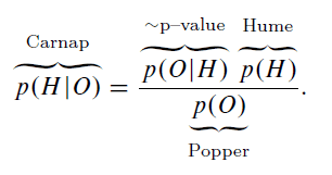
Understanding how to use the probability $p(H)$ to determine $p(H|O)$ is key—after all, induction is all about basing future expectations on experience. A boneheadedly simple theorem by Reverend Thomas Bayes published in the 18$^{\rm th}$-century provides a way of packaging up this experience, à la Goodman, and using it to compute the kind of probability that Carnap indicated as a route to confirmation. Starting with the tautology $p(O\cdot H) = p(H\cdot O)$ and using the definition of conditional probability, $p(H \cdot O) = p(H|O)p(O)$, we arrive at Bayes’ Theorem,
\begin{equation}
\label{bt}
p(H|O,\mathcal{M}) = \frac{p(O|H,\mathcal{M})p(H|\mathcal{M})}{p(O|\mathcal{M})},
\end{equation}
where I have referred $\mathcal{M}$, the underlying model that provides the functional relationship between the observations and the hypotheses—its role in the above expression is merely informational¹. Bayes’ Theorem facilitates the remarkable feat of transforming the probability of the evidence, $O$, given hypothesis, $H$, into the probability of the hypothesis, given the evidence. This quantity, $p(H|O,\mathcal{M})$, is referred to as the posterior odds of $H$ given evidence $O$. There is no strict verification or falsification—Bayes’ Theorem does not accept or reject $H$—it is a function of $H$ that assigns degrees of confirmation as Carnap sought. Bayes’ Theorem is not concerned with examining individual hypotheses—it provides instead a probability distribution over the entire hypothesis space. Generally, we seek the hypothesis that maximizes this function. The extent to which each hypothesis is confirmed depends on the strength of the data relative to what is known about $H$ beforehand, through the prior probability, $p(H|\mathcal{M})$; and on possible alternative explanations, through the probability of the data irrespective of hypothesis, $p(O|\mathcal{M})$. Let’s go through these quantities one by one.

First, the infamous prior: $p(H|\mathcal{M})$. This severely misunderstood quantity has caused much trouble for the Bayesian enterprise, often cited by dissenters as infusing what should be a concrete, no-frills computation with unnecessary subjectivity and speculation. Indeed, it does these things, but they are necessary. After all, to quote the late David MacKay, “You can’t make inferences without making assumptions!” [2]. The prior brings all of the world’s combined knowledge to bear on the assessment of a hypothesis. It’s where we include previous test results and guidance from theory. The prior is general—it must incorporate all prior knowledge, widely construed, across a varied portfolio of understanding. Great theories find support in many places: our knowledge of gravity is based on observations of the changing seasons and tides, the retrograde motion of Mars, and the twists of the torsion balance in the Cavendish lab. The prior is what embodies the repeatability of science, and separates the frivolous pseudoscientific proposals from the real meat. For example, the claim that a vastly diluted glass of beet juice protects against polio has virtually zero prior support from our understanding of molecular biology or physics, whereas our prior expectations that a vaccine will yield success rests on a significant body of biological knowledge. The prior helps enforce the burden of proof: claims with low prior odds (e.g. that homeopathy works) need overwhelming positive evidence to confirm with high posterior odds. The prior probability is where Goodman’s green and grue emeralds get sorted out, and where Hume ultimately finds his rationality for induction—human habit.

Next, the probability of the evidence, $p(O|\mathcal{M})$ (sometimes called the Bayesian evidence). This is the chance that we obtain the given dataset irrespective of the hypothesis,
\begin{equation}
\label{ev}
p(O|\mathcal{M}) = \sum_{H’}p(O|H’,\mathcal{M})p(H’|\mathcal{M}).
\end{equation}
It considers the possibility that other hypotheses could have given rise to the observed evidence. Consider what happens if there are many competing hypotheses, equally consistent with the data. Then, $p(O|\mathcal{M})$ is large, and the chance that any hypothesis $H$ is the true one, $p(H|O,\mathcal{M})$, is small. Meanwhile, if there are no alternative hypotheses, we find $p(H|O,\mathcal{M}) = 1$ with deductive certainty.

Lastly, the probability $p(O|H,\mathcal{M})$: it gives the chance that we’d expect to observe the evidence, $O$, under the assumption that the hypothesis, $H$, is true. In Bayesian vernacular, it is called the likelihood of $H$. You might remember this quantity from our earlier discussion of p-values, which are given by $p(O|\overline{H})$, where $\overline{H}$ is the null hypothesis, and proceeds by illegally equating $p(O|\overline{H}) = p(\overline{H}|O)$. We have in Bayes’ Theorem, by the added ingredients $p(H|\mathcal{M})$ and $p(O|\mathcal{M})$, the proper way to perform this inference. Bayes’ Theorem for the case of two hypotheses, $H$ and $\overline{H}$, is
\begin{eqnarray}
&=& 1 – {\rm p\mbox{–}value}\times\frac{p(\overline{H})}{p(O|H)p(H) + p(O|\overline{H})p(\overline{H})}.
\end{eqnarray}
When written this way, it is clear that the inference $p(H|O) = 1 – {\rm p\mbox{–}value}$ made so often in scientific studies follows only if $p(\overline{H}) = 1$, the assumption that the null hypothesis is certainly true. It is therefore impossible for $H$ to be anything other than false—$p(H|O) = 0$—and we again see the fallacy of using the p-value to confirm alternative hypotheses.

Now that we’ve introduced all the players, let’s see what Bayes’ Theorem can do. As an example, we’ll turn to the workhorse of statistics props—the urn filled with black and white balls. Suppose we are given an urn filled with 10 balls, $u$ of which are black and $10-u$ white. We draw $N=10$ balls at random, with replacement. $n_B=4$ of these balls are black. The task is to determine the number, $u$, of black balls in the urn. The number, $u$, is the hypothesis.

First, the probability of the data given the hypothesis,
\begin{equation}
\label{binom}
p(n_B|u,\mathcal{M}_1) = {N \choose n_B}f_u^{n_B}(1-f_u)^{N-n_B}
\end{equation}
follows a binomial distribution, where $f_u = u/10$. If we are ignorant about the number $u$, then our prior is noncommittal and uniform: $p(u|\mathcal{M}_1) = 1/10$ (there is either 1 black ball, 2 black balls, up to 10 black balls, each equally probable for a prior probability of $1/10$). The model, $\mathcal{M}_1$, refers to our description, $u$, of the number of black balls in the urn, together with our prior assumptions about $u$, namely that any number of black balls between 1 and 10 is possible with equal chances. The Bayesian evidence accounts for the chances that we’d select $n_B$ balls under each hypothesis, appropriately weighted by $p(u|\mathcal{M}_1)$ which is constant in this case,
\begin{equation}
p(n_B|\mathcal{M}_1) = \sum_u p(u|\mathcal{M}_1) p(n_B|u,\mathcal{M}_1).
\end{equation}
Calculating the sum gives $0.00042$, which will be important later. Because the Bayesian evidence and the prior probability are constants, the posterior odds are binomially distributed, proportional to Eq. (\ref{binom}). The posterior distribution is shown in Figure 1,

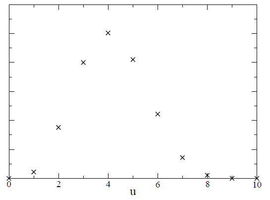
Fig 1. Posterior odds of $u$, the number of black balls in the urn, given that $n_B = 4$ black balls were drawn in $N=10$ trials with replacement.

As expected, the hypothesis $u=4$ is most likely, whereas the alternative hypothesis, say, $u=6$, has odds roughly 2-to-1 against.

But suppose we adopt a different prior. Say that we have some knowledge that suggests that there must be an even number of black balls in the urn. Maybe we have done some early experiments that support this assumption, or maybe we have some insight into the process by which the urns are filled. Either way, it’s possible to examine the same hypothesis, $u$, under a different set of prior assumptions—under a new model, $\mathcal{M}_2$. Now $p(u|\mathcal{M}_2) = 1/5$ for $u$ even, and $p(u|\mathcal{M}_2) = 0$ for $u$ odd. The Bayesian evidence is the sum Eq. (\ref{ev}) but now only over even $u$, giving $0.00054$. When we plot $p(u|O,\mathcal{M}_2)$, we find that the posterior odds are larger (for $u$ even) than the odds under the original prior, Figure 2,

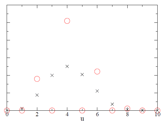
Fig 2. Posterior odds of $u$, the number of black balls in the urn, given that $n_B = 4$ black balls were drawn in $N=10$ trials with replacement. Black crosses assume a uniform prior overall $u$, and red triangles assume $u$ even.

What might this mean? Is Bayes’ Theorem telling us that the hypothesis $u=4$ under the second model is preferred by the data? Not necessarily: it’s generally possible to arbitrarily increase the posterior odds of a hypothesis by making that hypothesis more and more sophisticated. This is called over-fitting the data, and so the posterior probability distribution cannot be trusted with this determination.

To investigate this question more carefully, we can apply Bayes’ Theorem to the models themselves,
\begin{equation}
\label{ms}
p(\mathcal{M}|O) = \frac{p(O|\mathcal{M})p(\mathcal{M})}{p(O)}.
\end{equation}
Bayes’ Theorem not only calculates posterior odds over the space of competing hypotheses (in this case, the value of $u$), it also yields posterior odds over the space of competing models, $\mathcal{M}_i$. Notice something marvelous: the likelihood of the model, $p(O|\mathcal{M})$, is the denominator of Eq. (\ref{bt})—it is the Bayesian evidence! Unless we have strong a priori feelings about the various choices of model, then $p(\mathcal{M}_1) = p(\mathcal{M}_2)$ and the likelihood, and therefore the Bayesian evidence, is a direct measure of the posterior odds of the model. If we revisit the calculations of $p(u|O)$ above, the evidence under $\mathcal{M}_1$ is $0.00042$, while the evidence under $\mathcal{M}_2$ is $0.00054$. Indeed, $\mathcal{M}_2$ is preferred by the data. What is it about the second prior that results in a better “fit”?

It’s helpful to visualize the sample space of the urn to compare the two models. In Figure 3, each configuration is possible, with equal weight, according to the prior of $\mathcal{M}_1$, while only those in gray boxes—the even numbers of black balls—are possible under $\mathcal{M}_2$:

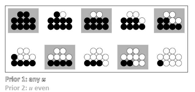
Fig 3. Graphical depiction of the configuration space of the urn problem: prior 1 includes all configurations, prior 2 includes only those with an even number of black balls.

Bayesian inference has a thing for minimal priors, both in the number of free parameters and the intervals over which they can range. The idea is that a model with a more economical parameter space is more exacting in its range of predictions, and hence, more easily falsified. This is exactly the sentiment behind Karl Popper’s notion of corroboration that was illustrated in Figure 2 of the previous note. Recall the importance that Popper ascribed to the empirical content of a hypothesis: the more lenient the hypothesis, the less it charges about the system under study. Popper argued that empirical content is inversely related to what he called the logical probability of the hypothesis [4], the idea being that we should select the least likely hypothesis given the data. This goes against the principles of Bayesian theory, which seeks the hypothesis with the greatest posterior odds. And so a sizeable rift opened across the field of scientific inference, with two opposing notions of what makes a hypothesis favorable. Both have an air of correctness about them: we do want our hypotheses to be precise and daring, but we also want them to be well-supported by the data. Can’t we have it both ways? I believe we can. Popper isn’t talking about the posterior odds, $p(H|O)$ when he argues for low probability. Rather, he has in mind what Figure 3 captures: that if we were to throw a dart at the prior sample space, we’d be less likely to hit those urn configurations belonging to model $\mathcal{M}_2$. It is in the prior space that we seek Popper’s low logical probability, not in the posterior odds of a particular hypothesis once the data arrive³. So Popper’s corroboration is a model comparison ($\mathcal{M}_1$ vs. $\mathcal{M}_2$) rather than a measure of support for a particular hypothesis within a given model (the value of $u$ within $\mathcal{M}_1$, for example). Bayes’ Theorem is a one-stop shop for both traditional confirmation and corroboration.

In conclusion, Bayes’ Theorem is the thread that connects the key aspects of prior knowledge, predictability, and goodness-of-fit to render a measure of confirmation—a posterior probability and corroboration of hypotheses. It is arguably our best method of scientific inference. Written down by Thomas Bayes in the 18$^{\rm th}$ century, it anticipated much of the work on induction and falsifiability that would challenge the greatest philosophical minds of the past three centuries: Hume, Carnap, Reichenbach, Quine, Hemple, Goodman, Popper, and so many more. Though incomplete, the various elements of Bayes’ Theorem have obvious champions:
Because of the problem of induction, we will never be certain of our scientific assertions or conclusions. Science is an enterprise that is perpetually imperfect in its compiled knowledge about the world because it must make guesses based on sometimes tenuous patterns and regularities in data sets that are always incomplete. Practical science proceeds by establishing theories as summaries of these regularities, but they are only approximations of the true structure. Eventually, with hope, anomalies or systematics will emerge in new data. Tantalizing and maybe a little maddening at first, they will reveal hints of new patterns and symmetries signaling a need to adjust the theory—maybe we falsify it or adjust it. The new theory that emerges is also transitional and ultimately wrong, but it is confirmed in the sense that it assumes the role of the new foundation, the next scaffold in the rise to the truth. It is selected just as a favorable trait in an evolving species—both seek an optimized form. As Popper said so well, “It is not his possession of knowledge, of irrefutable truth, that makes the man of science, but his persistent and recklessly critical quest for truth.”

References and Footnotes

[1] Statistical and Inductive Probability, Rudolph Carnap, in Philosophy of Probability: Contemporary Readings, Routledge (1955)
[2] Information Theory, Inference, and Learning Algorithms, David MacKay, Cambridge (2003).
[3] Conjectures and Refutations: The Growth of Scientific Knowledge, Karl Popper, Routledge (1963).
[4] The Logic of Scientific Discovery, Karl Popper, Routledge (1934).

¹Often when there is no risk of confusion, reference to the explicit model is suppressed; however, we will have cause to examine alternative models, and so we introduce this notation now. back
²In analogy with an actual scientific inquiry, knowing about the filling process might be like having some background knowledge from theory, or some other formal constraint on the system. back
³Popper also does not mean that the prior probability should be low, although he has made various arguments to this effect [3,4]. The prior probability of $u$ under $\mathcal{M}_2$ is larger, $p(u|\mathcal{M}_2) = 1/5$, than under $\mathcal{M}_1$, $p(u|\mathcal{M}_1) = 1/10$. This is because the prior probability is equally distributed across fewer states in the case of $\mathcal{M}_2$. The logical probability is based on the percentage of the configuration space permitted by the given model: $\mathcal{M}_2$, with half as many available configurations as $\mathcal{M}_1$, has half the logical probability. back