Learn Advanced Astrophotography Tips

 

“I’ve tried astrophotography and want to know how to improve.”

Here’s where I assume you are contemplating the purchase of a tracking mount- a motorized tripod. Far from being an afterthought, “A mount must relate to the telescope tube like a clockwork to the hand on the clock.” Purchasing a tracking mount represents a *significant* investment of time and money, with time being the more important- although you get what you pay for. Do you have time to spend a night outside at least twice a week for a year to learn how to use the mount? How much time do you want to spend setting up the gear and packing it up each night? Can you set up in your backyard, or do you need to drive somewhere? Mounts are electrically powered, so you will need either a battery or a power cord. Autoguiders, if you get one, require a computer, increasing the complexity. Mounts are very heavy and don’t lend themselves well to travel.

There are two basic types of motorized tracking mounts: alt-azimuth (Dobsonian) and equatorial. Equatorial mounts hold the camera steady in equatorial coordinates, while Dobsonian mounts hold the camera steady in horizon coordinates. One disadvantage of Dobsonian mounts is the requirement that the camera must also roll about the optical axis as the mount tracks; failure to perform this motion results in ‘field rotation’- the starfield appears to slowly rotate within the field of view. One disadvantage of equatorial mounts is the susceptibility to vibration. I have an equatorial mount.

One important transition when going to a motorized mount is finding that the maximum acceptable shutter time is not as clear-cut as before. For non-motorized tripods, the maximum shutter time can be easily determined for a particular DEC, and the ‘success rate’ of images will be nearly binary: less than this time, all the images are probably acceptable. More than this time, none of the images are acceptable. With motorized mounts, tracking errors introduce variability- there will be an ‘optimal’ maximum shutter time, where (say) 50% of your images are acceptable. This optimal shutter time can be 10-30 times what you can achieve with a static tripod, but if that amount of time is still too low (for very faint objects), you will need to improve your tracking mount’s accuracy.

Tracking accuracy:

Inaccuracies with an equatorial mount primarily stem from two sources- imperfect alignment with the polar axis, and periodic error of the motor drive.

Polar alignment error:

This is a misalignment between the RA rotation axis of an equatorial mount and the rotation axis of the earth. In the northern hemisphere, Polaris is currently 0.75° offset from the rotation axis (slightly more than 1 lunar diameter), so the equatorial mount is not precisely pointed at Polaris. I’m honestly not sure how equatorial mounts are aligned in the southern hemisphere- there’s no corresponding pole star. In any case, polar alignment needs to be as accurate as possible- tenths of a degree or better. I find that my mount settles during the first 30 minutes or so, I periodically re-check my polar alignment during the night and correct as needed.

Solution 1: polar alignment scope.

Most equatorial mounts have a space to insert a “polar alignment scope” fitted with an illuminated internal reticle which, when used, provides improved pointing accuracy (for either hemisphere), and it’s worth the added expense of having one.

Solution 2: Declination drift alignment

There is a method called ‘declination drift’ that can be used to really fine-tune polar alignment, but I haven’t tried it:

http://www.skyandtelescope.com/astronomy-resources/accurate-polar-alignment/

Periodic error correction:

Equatorial mounts need to convert a relatively fast rotation (the motor) to a very slow rotation (the camera). This is done with a set of gears, and manufacturing tolerances are such that the resulting camera motion is not precisely uniform; sometimes the camera moves too fast, other times too slowly. The effect repeats itself every complete revolution of the gearing (which occurs every several minutes), hence the term ‘periodic’. The periodic error manifests as star trails oriented exactly in the east-west (RA) direction. If your residual streaks are slightly curved or not exactly aligned with RA, your polar alignment is insufficient. 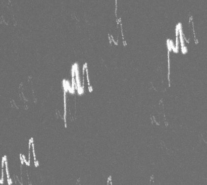Here’s an example of the effect- 50 consecutive 10-second exposures, taken at 800/5.6 (400/2.8 + 2X tele). Periodic error is up-down in this image, declination drift is left-right. 1 exposure (the last) is especially bad, but most of the exposures occur while there is relative motion between the sensor and starfield. You can also see my polar alignment is not perfect.

Solution: guiding.

This can be done manually (which is tedious) or automatically with a computer and second guide camera (which means more gear). Either way, you will be able to eliminate up to 80% of the periodic error if your mount can remember its training. After a round of manual guiding, I get this:

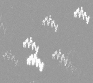
My polar alignment is still off, but the periodic error is about 50% less. As a result, my image acceptance rate increased from about 20% to 40%.

Field Rotation:

This is due to the use of horizon coordinates (Dobsonian mount). Again, the starfield will appear to rotate 15 arcsec/sec, but this rotation is about the optical axis; the number of residual star trails in long exposure will be determined by your image size. Field de-rotators are (optimally) rotating prisms that correct for this apparent motion. I don’t have much experience with field rotation, nor do I know what happens when a Dobsonian mount is not level with the horizon.

Magnitudes redux:

Let’s get serious about radiometric detectors (i.e. your digital sensor). To recap: apparent magnitudes are a logarithmic scale, the irradiance (also unfortunately referred to as ‘flux’) from two objects (I₁,I₂) is related to the magnitudes (m₁, m₂) by the formula:

I₁/I₂ = 2.512^(m₂-m₁). Each increment in magnitude is -1.3 Ev.

Your sensor, however, has (nearly) linear sensitivity with respect to irradiance. Converting apparent magnitude to irradiance is not simple, it requires information about the spectrum of the object. A detailed discussion is beyond the scope of this Insight, I’ll only provide rough guidance here. Since cameras are most sensitive in the visible band, it is appropriate to consider band-limited V-magnitudes, or the magnitude of objects if they are band-limited to the visible region (about 490 nm to 610 nm). There is a (reasonably) simple way to calculate the photon flux from V-magnitudes, using the unit ‘Jansky’ [Jy]. Here’s a summary table:

 

Object                              apparent magnitude    Jy                     photons sec^-1 m^-2          irradiance [W/m^2]

Sun                                   -26.74                            1.81E+14       4.37E+20                               1.30E+03

Full moon                        -12.74                            4.54E+08       1.10E+15                               3.27E-03

crescent moon               -6                                    9.14E+05       2.21E+12                               6.58E-06

Vega                                 0                                      3.64E+03       8.79E+09                               2.62E-08

stars in big dipper          2                                      5.77E+02       1.39E+09                               4.15E-09

eye limit (small cities)    3                                      2.30E+02       5.55E+08                               1.65E-09

eye limit (dark skies)     6                                      1.45E+01       3.50E+07                               1.04E-10

12                                   5.77E-02        1.39E+05                               4.15E-13

15                                   3.64E-03        8.79E+03                               2.62E-14

19                                   9.14E-05        2.21E+02                               6.58E-16

 

Remember when you struggled to properly expose a scene with a large dynamic range? Astrophotography amplifies that dynamic range problem by several orders of magnitude (pun semi-intended). Certain parts of the night sky (say, the Orion nebula) can have a dynamic range of close to 1,000,000:1- well beyond the capability of 8 bits to display, and even 16 bits to capture. And it gets worse: reported apparent magnitudes of extended objects make the objects seem brighter than they really are. The assignment of apparent magnitude to an extended object like a nebula or galaxy is done by assuming all of the collected light is incident on a single-pixel- the exact opposite of imaging. Unfortunately, there doesn’t seem to be a simple way to assign a magnitude to extended objects.

So what? Well, we can use the sensor as a radiometric detector and ‘measure’ stellar magnitudes. Let’s see how the above numbers translate to my sensor specifications:

http://www.sensorgen.info/

My sensor has a quantum efficiency of 47%. At ISO 500, I have a read noise level of 3.7 e-, a full-well capacity of 10329 e-, and a dynamic range of 11.5 Ev. Let’s first check these numbers for consistency- 2^11.5 = 2900, which seems low- for an Ev = 13.35; 2^13.3 = 10400, close to the full-well capacity.   But we didn’t account for reading noise- because of reading noise, my camera can reliably distinguish only 2800 distinct increments of charge, which gets me close enough to 11.5 Ev.

To recap:

A single 400/2.8, 15s ISO-500 image results in an average grey-level background value of 3500, and a magnitude 14.1 star generates a grey-level of 4542 (1242 levels above background). These per-pixel values correspond to 2200 e- and 2860 e-. Now let’s see what grey levels we expect to measure based on the table above.

According to the above table, imaging a 14.1 magnitude star should generate 550 e- per pixel, far below the corresponding grey values I reported above…. What?

I haven’t accounted for the background illumination yet. The background is a diffuse source, not a point source, so the approach differs. We begin with luminance rather than irradiance. The light-polluted (moonless) night sky has a luminance of about 0.1 mcd/m². Turning the crank requires knowing the angular field of view (per pixel) and the spectral sources of light. The field of view is straightforward, and assuming that light pollution is primarily from Sodium lamps, this converts to 3.4*10^-14 J/pixel on a 15-second exposure through my lens. This is ‘apparently equivalent to a magnitude 10.8 star.

But I overestimated- for a point source, the received power is averaged over the PSF area, but not the case for diffuse illumination. Accounting for the PSF area the background illuminance now has the ‘equivalent apparent magnitude’ of a magnitude of 12.1 star. The excess 570 e- from a magnitude 14.1 star is now slightly above the background, as expected.

Let’s pause to contemplate the ability to measure fJ of energy with a commercial camera. Seriously- today, you can image objects that even 30 years ago required professional observatories to see.

So, what is the lower magnitude limit I can expect? It depends on the total exposure time and the ability to separate stars from the background. Let’s say that I require each 15-second frame to have 4 excess e-/pixel over the background, just above the read noise threshold- that correlates to a magnitude 19 star. Over a 2-hour exposure, a magnitude 16 star will provide 760 excess e-/pixel, and I may be able to pull out a magnitude 18.5 star (76 excess e-/pixel). If I reduce my tracking error down to where I can acquire 30-second (or 1 minute) exposures, I expect my detection limit to decrease accordingly. Verifying these limits is not easy since star catalogs don’t have too many faint stars listed.  And again, using low surface brightness galaxies (or other extended objects) is problematic due to the way apparent magnitude is defined. In any case, it is reasonable to attempt to detect occultations:

http://iris.lam.fr/wp-content/uploads/2013/08/1305.3647v1.pdf

Tone mapping, redux:

One crucial point about > 8-bit images: your monitor is not built to display more than 8 bits of intensity (per channel). The only way to reproducibly post-process high SNR images to operate on quantitative metrics of your image (say, adjust a pixel brightness histogram with a gamma correction).

In terms of post-processing, using logarithmic tone mapping is how to best tone map a high dynamic range image (covering say, 10 stellar magnitudes) into a linear 8-bit image. Adjust ‘gamma’ to adjust image contrast. This is similar to Dolby noise reduction: the signal is compressed and amplified into the upper range and then threshold the noise.

http://www.cambridgeincolour.com/tutorials/dynamic-range.htm

As I mentioned above, thinking in terms of an H&D curve is helpful. However, the optical density scale (‘D’) does not have to be logarithmic- increased dynamic range compression can be obtained by mapping log(log(D)) to H, faint nebulas are best amplified with that functional relationship. Similarly, dynamic range compression can be lessened by using other functions of D: I obtain excellent results of starfields by mapping the cube root of D onto H. Just remember- the more dynamic range compression, the larger your FWHM is going to be.

Special note: there is a useful alternative magnitude scale specially designed for faint objects, the ‘Asinh magnitude scale”:

https://arxiv.org/abs/astro-ph/9903081

Color balancing:

I struggle with this and have to perform image adjustments ‘by instrument’, not ‘by eye’ in order to get consistent results. Because the tone map is nonlinear, at least 3 ‘setpoint’ intensities are required to permit accurate white balancing: one for black, one for white, and one mid-tone neutral grey. Without the midpoint, midtones can span the hue range from purple to green, even if the white and black are neutral. Channel-by-channel gamma correction can be used to bring the midtones into balance, but there’s not much I can offer for guidance. As a possible alternative, there are programs that can access online astrometry databases and calibrate your images:

http://bf-astro.com/excalibrator/excalibrator.htm

I have yet to use this, it seems rather involved.

Deconvolution:

Under certain conditions (linear-shift invariant systems), the image is given as the object field convolved with the PSF. Linear shift-invariance is strictly violated for sampled imaging systems, but in many cases, it still serves as a useful approximation. The idea, then, is to ‘divide’ by the PSF and recover a higher-fidelity representation of the object field. The computational aspects are non-trivial since the PSF has many zeros, so I’ll leave a detailed treatment out. Suffice to say, deconvolution can be used to improve the overall quality of your image, but don’t expect a huge improvement.

Unsharp masks:

This is a simple way to boost abrupt changes in intensity (‘sharpen’). Duplicate your image and blur it with a few-pixel (try between 5 and 10) wide kernel. This blurred image is then weighted by a factor (say, multiply by 0.3) and subtracted from the original. The low-frequency intensity components are (slightly) diminished and the high-frequency components corresponding to edges are (slightly) amplified.

CLAHE:

Another way to boost contrast is ‘contrast-limited adaptive histogram equalization. The method boosts contrast by computing and equalizing local histograms. The result is that small variations in intensity are amplified more than large variations in intensity. There are some side-effects to this method that make it less satisfactory for extended objects and very dense clusters. It works great on starfields.

https://en.wikipedia.org/wiki/Adaptive_histogram_equalization#Contrast_Limited_AHE

Background subtraction:

Fast lenses suffer from fall-off due to the entrance pupil area varying with view angle- the effective area decreases as the viewing angle moves away from normal. In stacking programs, you can also provide several ‘flat’ images that are used to correct for fall-off, ‘flattening’ the image background. Flats are images of a uniform intensity field of view. Flats aren’t too hard to acquire- a white LCD/computer monitor can be used as a uniform source. Flats can reduce the background variation by (in my experience) up to 95%. Then the background is literally subtracted from the image. I have found that my ‘flat’ reference needs a little (gamma) tweaking for optimal performance.

Background subtraction works really well when there is good length scale separation: stars maybe 5 pixels wide, but the sky background varies with a length scale of 100 pixels (or more). Then local averaging, with an intermediate length scale, say 50 pixels, in this case, will efficiently remove well over 99% of the background. Unfortunately, when imaging extended objects such as galaxies and nebulae, there isn’t such a large separation in scales and the above routine will fail.

An alternative, to remove background variances that cover length scales approaching the whole image (a ‘DC component’), is to subtract an image that has been blurred using a kernel size of ~1000 pixels from the original. Don’t forget to first add a border with the value set close to the median grey value, wide enough to accommodate the kernel.

Noise reduction:

Here, ‘noise’ is the term given to high spatial-frequency intensity fluctuations. There are many ways to reduce noise, including specialized programs. Often, a Gaussian smooth filter with a 0.6 pixel-wide kernel is good enough.

A clever way to reduce noise is to re-slice your RGB stack. Conceptually, this is closely related to ‘squeezed states’. Seriously. What I mean is that stacking programs will produce an image stack with (R,G,B) channels because the is the output of the sensor. Per-channel noise is (essentially) equally distributed among the three channels. There is an alternate color space called Hue-Saturation-Brightness (HSB). Converting an RGB stack into a HSB stack will result in the noise being equally distributed into the HSB channels, but it is easy to reduce noise in the H and S channels: neighboring pixels should have similar Hue, and the overall image should have the same saturation. Thus, smoothing/despeckling on H and setting S to a constant value nearly eliminates 66% of the overall noise. If you like, adjust the B channel as well to improve levels and contrast. Converting back to the RGB stack will result in a significant improvement.

Something fun: astrospectrophotography

Now that you are able to take 10+ s exposures, you could see what happens when you place an inexpensive transmission diffraction grating into the optical path, for example where the filters go. See if you can measure the spectral differences between the major planets or bright stars.

Something else: stitched panoramas

Why be limited by your lens’s field of view? Stitch a few frames together for a really impressive image. I have found that the individual frames need to have a similar color balance (obvious!) and SNR (not so obvious!). Doing all post-processing ‘by instrument’ rather than ‘by eye’ helps everything stay constant.

Missed the first two parts?
Part 1: Introduction Astrophotography
Part 2: Intermediate Astrophotography