
An Example of An Accurate Hooke’s Law Laboratory
Table of Contents
Learning Objectives
- Gain confidence and experimental care in making accurate measurements.
- Understand the relationship between force and spring stretch.
- Use a neat and orderly lab notebook in which data are recorded.
- Execute a specific experimental procedure to test a specific hypothesis.
- Analyze the acquired data with a spreadsheet and graphing program to test the hypothesis.
- Explain in one’s own words whether the experimental data supported the hypothesis.
Introduction
Robert Hooke was a 17th-century scientist who made notable discoveries in a wide range of fields from astronomy to biology (discovery of the cell). His discovery of the linear relationship between the extension of a spring and the applied force has broad application in engineering and physics because it has been shown to apply in a wide array of circumstances for sufficiently small displacements. Most of Hooke’s discoveries resulted from careful observations and measurements.
Hypothesis: Spring stretch and applied force are linearly related. This hypothesis can be tested by hanging known masses (which create known downward forces) to a spring and measuring the resulting displacements. The slope of the line from plotting Force (in N) vs. position (in m) is a characteristic of the spring known as the spring constant (in units of N/m).
Note, that Hooke’s law is most commonly expressed as a direct proportionality between force and spring stretch. However, many simple coil springs are wound such that the coils physically prevent the spring from contracting all the way to the true unstretched position that would correspond to zero displacements for zero applied force. Consequently, it takes some finite applied force to overcome the resulting internal tension and produce a measurable displacement. To accommodate these springs, it is convenient to frame the hypothesis as a linear relationship rather than a direct proportion. This also allows students to simply record the position for each hanging weight rather than computing the displacement from the position corresponding to zero hanging weight.
Method
Materials
* A spring that has a significant and easily measurable stretch with the available masses. Here, a composite spring is constructed from 3 #84 springs arranged in series. These springs were purchased at an Ace hardware store.
* Electronic balance (if masses are unknown).
* A range of test masses (6-8) that can be hung to stretch the spring. Masses should have a range of values so that the heaviest mass is 3-4 times the lightest mass, and the range has (approximately) equal steps over the interval.
* A rigid hook, bar, rod, or other support from which spring may be suspended as masses are hung.
* A ruler, meter stick, or another length scale that may be hung vertically and rigidly behind the stretched spring for accurately measuring the position of the lower end of the stretched spring. Easy to read 1 mm tic marks are preferable.
* A lab notebook for recording data.
* A computer, plotting program, and spreadsheet for analyzing data.
Procedure for Experiment
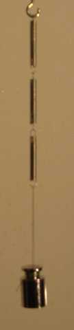
Prepare a page in your lab notebook with two columns. The first column is the hanging mass (in grams). The second column is the position of the lowest edge of the spring (in mm). The number of rows should correspond with the number of hanging masses (between six and eight). Set up your spring as shown in the figure to the left. The spring should be hung from rigid support that does not move as masses are applied. There needs to be a length scale behind the stretched spring for determining the spring position for each of a range of applied masses. If masses are not known, they need to be determined and recorded using the electronic balance.
Beginning with the lightest mass, hang each mass in turn from the spring. As each mass is hung, dampen the motion as best you can with your hand until the motion stops or becomes small enough that an accurate position measurement can be made. Record the position of the lowest portion of the spring in a table on the line corresponding to the mass. It is important to use the same part of the spring for this position measurement. The figure below shows the measurement for the spring position in our lab for the 150 g mass. Note some effort was taken to align the camera looking horizontally at the bottom spring coil for an accurate measurement.
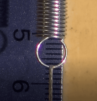
Likewise, it is essential to position your eye looking as near as possible to exactly horizontal when making the position measurement. Looking slightly upward or downward when lining up the position of the spring coil with the position scale will introduce parallax error. Repeat this measurement for each of your test masses until the table in your lab notebook is complete.
Procedure for Analysis
Make four columns in a spreadsheet with headings of Mass (g), Position (mm), Position (m), and Force (N). The first two columns contain the numbers for your original measurements, exactly the same as they are recorded in your lab notebook. The third column contains the position converted to meters with an appropriate spreadsheet formula, something like = B3/1000 (assuming the position in mm was in cell B3). The fourth column computes the applied force for each given mass, with a spreadsheet formula something like = A3*9.81/1000 (assuming the mass in g was in spreadsheet cell A3).
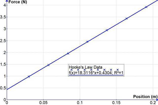
Now, copy the third and fourth columns for Position (m) vs. Force (N) (data only, no headers) into Graph.exe (downloadable for free from https://www.padowan.dk/download/ ) or other suitable graphing program and make a scatter plot of the data. Adjust the level of zoom as needed and take care to properly label the horizontal (x) axis as Position (m) and the vertical (y) axis as Force (N). You may also make other aesthetic adjustments to improve the appearance of the graph. Now, use the trendline menu option to insert a linear trendline. Do not check the box setting the y-intercept to zero. Make aesthetic adjustments to improve the appearance of the graph. Save your work as a graph file. Now, you may also save the graph as an image so that it can be imported into your lab report later. The slope of the trendline provides an accurate estimate of the spring constant, k, of your spring. It has units of N/m (newtons per meter) and is a characteristic of the spring.
Figure: Force vs. position for our Hooke’s law experiment, along with the best fit line.
NOTE TO TEACHERS: The instructions above are a compromise to obtain the spring constant directly as the slope of the best fit line. Some teachers prefer to teach their labs always plotting the dependent variable on the vertical axis. If you prefer students to plot position vs. Force (position on the vertical axis), the slope of the best fit line will yield the reciprocal of the spring constant (in m/N), and an additional calculation will be needed to compute the spring constant. This approach is also more rigorous statistically since the least-squares method works better with smaller uncertainties in the x variable. (In this experiment, the applied forces probably have smaller errors than the measured positions.)
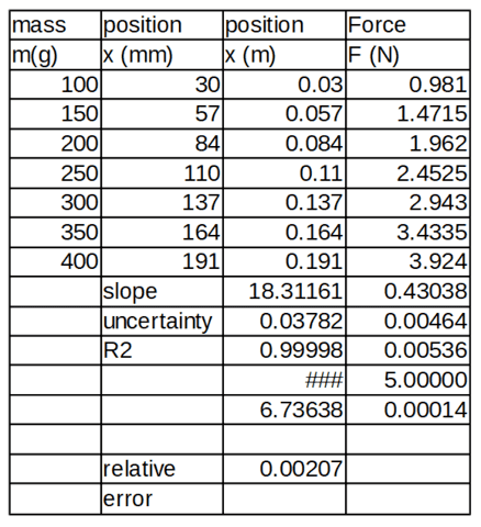
Now, the fancy stuff. Enter the LINEST spreadsheet call to repeat the least-squares fit in the spreadsheet. Something like =LINEST(D3:D9, C3:C9,1,1) in a cell in column C with plenty of room below and in the D column next to it. Hit CTRL-SHIFT-ENTER rather than just ENTER. This will make the full array of output visible rather than just one element. Several elements that are output will have important interpretations that are noted in the table.
Label resulting cells appropriately as slope, uncertainty, and R^2 (R squared) as shown in the table. Then compute the relative uncertainty in the spring constant (slope) as the ratio of the uncertainty to the slope and label it appropriately.
The rationale for Extended Analysis
The goal of low-cost quality experiments tends to put more of the burden on the analysis side than on the experiment side because most people have already invested in computers and the analysis software can be obtained for free. Further, extended and careful analysis is excellent training in scientific thinking, builds skills that will be useful in college, and reinforces skills that will increase scores on standardized tests like the ACT. Don’t give the analysis efforts short shrift. These tools and techniques will be used often and careful attention to these details is essential preparation for later laboratories.
Results (50 points total)
Your results should a well ordered and labeled table (15 points), as well as a figure (15 points) with the trendline and data produced in a graphing program. The above figure and table are illustrative examples, but it is essential that yours are created with your own original data. Pay attention to formatting and communication. The Table needs to be properly captioned and should also have a paragraph of text (10 points) describing its contents, but saving discussion relative to the hypothesis for the discussion section. Pay careful attention to include all the specific accuracy estimates in your table that are shown below. These are important in the discussion of whether the hypothesis is supported, and the uncertainty in the spring constant may also be important in later lab testing predictions for the period of simple harmonic oscillators. The Figure also needs to be properly captioned and should be described in a paragraph of text (10 points).
Table 1: Data and analysis for Force vs. Position for our Hooke’s Law experiment.
Discussion (50 Points)
Your written discussion should be from 1 to 3 paragraphs discussing the following questions in complete sentences:
* Was your hypothesis supported? Why or why not? (20 points)
* What was the relative uncertainty of your spring constant? (10 points)
* Other than the accuracy of the electronic balance, what else may have caused variations in your measurements? (10 points)
* Can you say your hypothesis was proven (or disproven)? Or is it better to say supported (or unsupported)? (10 points)
Note on lesson plans:
Teachers should consider a multi-day approach to this lab. Day 1: Discuss the theoretical background and read the lab instructions. Day 2: Perform the experiment. Day 3 (possible homework): Analyze the data. Day 4 (best as homework): Write lab report. A good lab science course uses 30-40% of class time on lab activities and completes at least 15 different lab experiments in a school year.
I grew up working in bars and restaurants in New Orleans and viewed education as a path to escape menial and dangerous work environments, majoring in Physics at LSU. After being a finalist for the Rhodes Scholarship I was offered graduate research fellowships from both Princeton and MIT, completing a PhD in Physics from MIT in 1995. I have published papers in theoretical astrophysics, experimental atomic physics, chaos theory, quantum theory, acoustics, ballistics, traumatic brain injury, epistemology, and education.
My philosophy of education emphasizes the tremendous potential for accomplishment in each individual and that achieving that potential requires efforts in a broad range of disciplines including music, art, poetry, history, literature, science, math, and athletics. As a younger man, I enjoyed playing basketball and Ultimate. Now I play tennis and mountain bike 2000 miles a year.


Leave a Reply
Want to join the discussion?Feel free to contribute!