Differential Equation Systems and Nature

Abstract

“Mathematics is the native language of nature.” is a phrase that is often used when it comes to explaining why mathematics is all around in natural sciences, especially in physics. What does that mean? A closer look shows us that it primarily means that we describe nature by differential equations, a lot of differential equations. There are so many that it would take an entire encyclopedia to gather all of them in one book. The following article is intended to take the reader through this maze along with examples, many pictures, a little bit of history, and the theorem about the existence and uniqueness of solutions: the theorem of Picard-Lindelöf.

A Glimpse of Our Descriptions of the World

It all began with Isaac Newton in 1687, or if we are picky, with Gottfried Leibniz during his stay in Paris 1672-1676 [34]. The reference to Paris is more than a side note since it will be especially French mathematicians who will develop the field of analysis in the following centuries to the state we know today. Joseph-Louis Lagrange, Pierre-Simon Laplace, Adrien-Marie Legendre, Augustin-Louis Cauchy, and Pierre-Alphonse Laurent are names we take for granted in everyday use. Charles Briot and Jean-Claude Bouquet coined the term of a holomorphic function in 1875 and the family of differential equations
$$
x^my’=f(x,y)
$$
carry their name. Other great contributors have been the Bernoulli family (Jakob, Johann, Daniel), Carl-Friedrich Gauß, George Gabriel Stokes, Marius Sophus Lie, and Amalie Emmy Noether to name a few. They all set milestones in mathematics and paved the way.

 

Of course, there has been important mathematics before the seventeenth century, as there has been important physics before Newton. Euclid of Alexandria and Archimedes of Syracuse lived in the third century B.C.! But if we look at the main subjects that we need today to describe nature, then we will end up with power series and forces.

Physics

It all began with Isaac Newton in 1687.
$$
F \;\sim\;\ddot{x}
$$
is nowadays the definition of a force. And it is a differential equation! The equation also tells us what happens without a force, namely that there is no change of motion $\dot{v}$ either, i.e. motion is conserved under the absence of forces
$$
F =0\;\Longleftrightarrow \;\ddot{x}=\dot{v}=0.
$$
Emmy Noether [1],[2] showed 231 years later that every conserved physical quantity corresponds to invariants of differential expressions. For example, James Clerk Maxwell introduced in 1864 his equations of electromagnetism which are all differential equations. Electromagnetism is a theory of the corresponding vector fields.
\begin{align*}
\vec{\nabla} \times \vec{H}=\vec{j}+\dot{\vec{D}}\; &, \;
\vec{\nabla} \times \vec{E}=-\dot{\vec{B}}\\
\vec{\nabla} \cdot \vec{D}=\rho\; &, \;
\vec{\nabla} \cdot \vec{B}=0
\end{align*}
Albert Einstein [3] even described the whole cosmos in 1915 by the differential Einstein Field Equations
$$
R_{\mu \nu }-{\frac{1}{2}}g_{\mu \nu }R+\Lambda g_{\mu \nu }={\frac{8\pi G}{c^{4}}}T_{\mu \nu }.
$$
These are outstanding results without any doubt. The example of forces in classical, say non-relativistic physics and Noether’s theorem, however, show that there are more examples to expect.

What the Taylor series is for mathematicians
$$
f(x)=\sum_{n=0}^\infty \dfrac{(x-x_0)^n}{n!}\cdot \left. \dfrac{d^n}{dx^n}\right|_{x=x_0}f(x)
$$
is the harmonic oscillator for physicists
$$
{\ddot{x}}+\omega^{2}\,x=0.
$$
They appear every year during the study of mathematics, resp. physics in new variations and contexts, and both are differential expressions. Balthasar van der Pol found in 1927 while studying vacuum tubes an oscillator with non-linear damping and positive feedback
$$
\ddot{x}-\varepsilon (1-x^{2}){\dot{x}}+x=0
$$
that does not allow a closed solution. Most systems aren’t as nice as waves
$$
\ddot{x}\sim \nabla^2 x
$$
or the heat equation (Jean-Baptiste Joseph Fourier, 1822)
$$
\dot{x}\sim\nabla^2 x.
$$
The holy grail of differential equation systems among the not-so-nice systems are the Navier-Stokes equations
$$
{\displaystyle \overbrace {\underbrace {\frac {\partial \mathbf {u} }{\partial t}} _{\begin{smallmatrix}{\text{Variation}}\end{smallmatrix}}+\underbrace {(\mathbf {u} \cdot \nabla )\mathbf {u} } _{\begin{smallmatrix}{\text{Convection}}\end{smallmatrix}}} ^{\text{Inertia (per volume)}}\overbrace {-\underbrace {\nu \,\nabla ^{2}\mathbf {u} } _{\text{Diffusion}}=\underbrace {-\nabla w} _{\begin{smallmatrix}{\text{Internal}}\\{\text{source}}\end{smallmatrix}}} ^{\text{Divergence of stress}}+\underbrace {\mathbf {g} } _{\begin{smallmatrix}{\text{External}}\\{\text{source}}\end{smallmatrix}}}.
$$
They are named after Claude Louis Marie Henri Navier and George Gabriel Stokes, and they describe the behavior of fluids and gases like water, air, or oil. They are therefore important in the development and design of ships, airplanes, and cars. They can only be solved numerically in their discrete version. There are no exact analytical solutions for these complicated applications. The Navier-Stokes equations are also a mathematical challenge because we do not know whether there is an everywhere-defined, smooth, and unique solution for the general three-dimensional case at all. This is one of the seven-millennium prize problems [4]. The Poincaré conjecture is considered to be solved by Grigori Perelman (2002,2003) so we should probably better speak of the six-millennium prize problems of the Clay Mathematics Institute.

 

The language of physics, at least the aspect of it with which we are concerned, namely differential geometry, is full of designations for differential expressions. There is of course the simple differentiation that leads to the differential operator
$$
\dfrac{d}{dx}
$$
The point why it carries its own name other than differentiation is the point of view: we transform one function $x\mapsto f(x)$ to another function $x\mapsto f'(x)$ rather than computing slopes. Its multivariate counterpart is the Nabla operator
$$
\vec{\nabla }=\left({\dfrac{\partial }{\partial x_{1}}},\ldots ,{\dfrac{\partial }{\partial x_{n}}}\right)$$
that produces the gradient vector of a function. It leads to the Laplace operator
$$
\Delta f=\nabla \cdot (\nabla f)=(\nabla \cdot \nabla )f=\nabla^{2}f
$$
when applied twice. It deserves its own name since it appears in another designation, the Schrödinger operator
$$
\dfrac{\hbar^{2}}{2m}\Delta +V
$$
and the d’Alembert operator
$$
\Box=\dfrac{1}{c^2}\dfrac{\partial^2}{\partial t^2} -\Delta \,.
$$
Even the Hodge star operator
$$
{}^\ast \colon \Lambda ^{k}(V^{*})\rightarrow \Lambda ^{n-k}(V^{*})
$$
that only transforms vectors in Graßmann algebras, at first sight, is an operator between cotangent spaces at second sight and thus an operator in differential geometry, too. There are also named differential equations or better, differential formalisms that carry specific names like the Lagrangian or Euler-Lagrange equation
$$
\dfrac{d}{dt}\dfrac{\partial L}{\partial \dot{q}}- \dfrac{\partial {L}}{\partial q}=0
$$
The importance of differential expressions in the description of physics is reflected in the language of physics. However, I promised you the description of the world and although we already had the description of the cosmos, and physics is per definition all of nature, let’s have a look into other fields of science.

Other Sciences

We find differential equations even in Chemistry which is by nature a discrete world, e.g. the reaction equation of three substances [5]
$$
\dot{x}(t)=K(A-x)(B-x)(C-x)
$$
This looks admittedly a bit artificial but differential equations have been really modern in 1889. And to be fair, the balance equation in a Bachelor’s paper from 2010 [6] in chemistry is not so much of a difference. My professor for differential systems used to say that the entire world is discrete if you only look closely enough. Nevertheless, he taught us how differential equation systems can be approached and in some cases solved. So differential equation systems found their way even into chemistry.

The situation changes completely as soon as we consider stochastic differential equations, i.e. derivatives of probability density functions $P(x,t).$ This opens up the door for a whole variety of applications, especially in economics. The Fokker-Planck differential equations named after Adriaan Daniël Fokker and Max Planck
$$
\dfrac{\partial }{\partial t}P(x,t)=\underbrace{-\dfrac{\partial }{\partial x}\left[A(x,t)P(x,t)\right]}_{\text{drift}}+\underbrace{\dfrac{1}{2}\dfrac{\partial^2 }{\partial x^2}\left[B(x,t)P(x,t)\right]}_{\text{diffusion / fluctuation}}
$$
are widely used in economics, e.g., in forex trading [7], equilibrium models for insider trading [30], on transition processes of income distributions [8], and more. The related Black-Scholes differential equations
$$
\dfrac{\partial C(x,t)}{\partial t}=-\dfrac{1}{2}\sigma^2x^2 \dfrac{\partial^2 C(x,t)}{\partial x^2}-rx\dfrac{\partial C(x,t)}{\partial x}+rC(x,t)
$$
named after Fischer Black and Myron Samuel Scholes are considered a milestone in option prizing [9]; $C(x,t)$ represents the prize of the derivatives. Another example of differential equations in economics is Kaldor’s growth model [10] from 1957 named after Káldor Miklós
$$
\dot{y} \sim c(y) +\dot{k} – y +k_0
$$
where $y$ is the gross national income, and $k$ the national capital stock. Even car traffic can be modeled by differential equations, the traffic equation, a non-linear hyperbolic wave equation for flow $f(x,t)$ and density $\varrho(x,t)$
$$
\dfrac{\partial }{\partial t}\varrho(x,t) + \dfrac{\partial }{\partial \varrho}f(\varrho (x,t))\cdot \dfrac{\partial }{\partial x}\varrho(x,t)=0\,.
$$
Of course, economics, macro- as well as microeconomics also use the wide areas of game theory [11], and control-theory [12],[13]. Differential equation systems play a central role in both fields. Let me mention the mean-field game theory as an example. It is the study of strategic decision-making by small interacting agents in large populations.
\begin{align*}
\partial u_t-\nu \Delta u+H(x,m,Du)&=0\\{\partial m_t}-\nu \Delta m-\operatorname{div}(D_{p}H(x,m,Du)m)&=0\\ u(x,T)-G(x,m(T))&=0
\end{align*}
The similar name to mean-field theory in physics is intended.

An often overlooked application of differential equation systems is timber management, on local as well as nationwide levels. The timber industry is almost predestined for differential equations: long-term investigation periods, natural growth with human disturbances, and yield optimization under constraints. D.B. Müller introduced a regional model that he called XYLOIKOS in his dissertation [14] that is based on $200$ years of data. His standard version of the model consists of $221$ coupled non-linear integral and differential equations, $182$ parameter functions, and $371$ single parameters! The corresponding simulation has been realized H.P. Bader and R.Scheidegger in Rocky-Mountain-Basic, 1996 [15].

 

Considering the complexity of differential equation systems in the regional timber industry, imagine the size of climate models! I recommend that interested readers look for lecture notes on university servers, e.g. [16], and the literature mentioned there. The first general circulation model by Manabe and Wetherald dates back to 1967 [17], and we have been progressing ever since. We can’t even come close to going into climate models here, so I just want to mention Daisyworld – with a blinking eye.

\begin{align*}
\dot{A}_w&=\left(\beta_wA_g – \chi \right)A_w\\
\dot{A}_b&=\left(\beta_bA_g – \chi \right)A_b\\
A_g&=1-A_w-A_b
\end{align*}
James Lovelock and Andrew Watson created a computer simulation in 1983 [18] in order to support the Gaia paradigm which says that the biosphere of a planet, our planet, forms a synergistic and self-regulating, complex system that helps to maintain and perpetuate the conditions for life on a planet. Their hypothetical planet had only two life forms, black and white daisies, and is otherwise similar to Earth [19]. They mainly investigated the size of the areas where those daisies grow and their albedo effect. Both, the Gaia paradigm as well as the simplifications of the model were subject to criticism and we must not forget the time, will say, the increased computer capacity we gained in the meantime.

A perfect moment to remember Moore’s law: the number of transistors on microchips doubles every two years [20].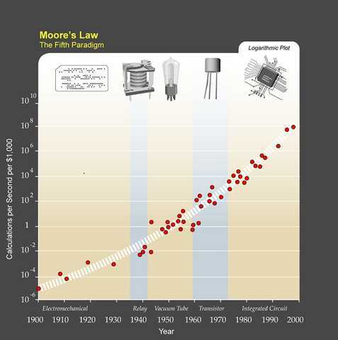

 

Biology

Any differential expression is a formula about change, often according to a time variable. And biology is the field of natural sciences where all is about change, namely growth.
$$
\dot{x}\sim x
$$
is the simplest and most basic formula of growth. Its solution is
$$
t\longmapsto x(t)=e^{at}
$$
and therefore called exponential growth, cp. [21]. It describes for example the unconstrained growth of bacteria, or Moores’s law. However, nothing in nature is without constraints. We consider thus in a first step the logistic growth
$$
\dot x \sim x\cdot (c-x)
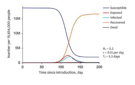
$$
with a capacity limit, e.g. the size of the Petri dish. But other than a bacterium in a Petri dish are bacteria in the wild not independent from another, or other changing parameters. This means, that the better we want to describe reality, the more we have to consider coupled systems with feedback, be it positive (virus infection) or negative (declining resources). The previous examples showed this. One of the more famous classes of differential equation systems in nature are SIR or Kermack-McKendrick-models, especially with Covid in mind [22],[23]
\begin{align*}
\dfrac{\mathrm{d} S}{\mathrm{d} t}&=\nu \,N-\beta \dfrac{S\,I}{N}-\mu \,S\;,\\[6pt]
\dfrac{\mathrm{d} I}{\mathrm{d} t}&=\beta \dfrac{S\,I}{N}-\gamma \,I-\mu \,I\;,\\[6pt]
\dfrac{\mathrm{d} R}{\mathrm{d} t}&=\gamma \,I-\mu \,R\;.\\
\end{align*}

SIR models are intended to describe outbreak, course, and the end of epidemics and pandemics and were introduced by William Ogilvy Kermack and Anderson Gray McKendrick in 1927 [24]. The three quantities under consideration are the number of Susceptible individuals, the number of Infectious individuals, and the number of Removed (and immune) or deceased individuals. The extensions of the model that also take the number of Exposed individuals into account are called SEIR models [25]. The coefficients reflect recovery and infection rates, and general birth and death rates. They do not depend on time, which is a significant simplification compared to real-life pandemics where varying types of a virus occur.

Predator-Prey Model

The differential equations for a system with a predator and a prey population have been set up independently by Alfred James Lotka [26] in 1925 and Vito Volterra [27] a year later. The Lotka-Volterra models work quite well for two or three species. Furthermore, they have the big advantage that we can draw, explain, solve – more or less – and test them. That’s why they show up in every textbook that deals with coupled differential equation systems and consequently, here, too. The basic idea behind the equations is, and this is a well-documented phenomenon in countless biological situations, that a population of predators thrives when prey is there in abundance, which declines the population size of prey, so that predators are forced to have fewer offspring, and the population of prey can recover until the cycle starts again. The two coupled differential equations are
\begin{align*}
\dot{x}(t)&=x(t)\left(\alpha -\beta y(t)\right)\\
\dot{y}(t)&=-y(t)\left(\gamma -\delta x(t)\right)
\end{align*}
where $t$ is the time variable, $x(t)$ the population size of prey, and $y(t)$ the number of predators. The coefficients are the parameters. They must be adjusted to the situation under investigation. $\alpha >0$ is the birth rate of prey on ideal conditions, $\beta>0$ the death rate per predator. $\gamma >0$ is the death rate among predators, and $\delta$ the reproduction rate of predators per prey. If I remember correctly, then my professor mentioned wolves, mountain hares, and caribous in Nova Scotia as a working example. However, it will be sufficient for demonstration reasons to choose some fantasy values that ensure nice pictures. Hence we will consider the equations
\begin{align*}
\dfrac{dx(t)}{dt}=\dot{x}(t)&=10x(t)-2x(t)y(t)=(10-2y(t))\cdot x(t)\\[6pt]
\dfrac{dy(t)}{dt}=\dot{y}(t)&=-7y(t)+x(t)y(t)=(-7+x(t))\cdot y(t)
\end{align*}
If we eliminate $dt$ and integrate on both sides, then
$$
y(t)^{10}e^{-2y(t)}=k\cdot x(t)^{-7}e^{x(t)}\, , \,k=e^C>0
$$
which transforms to the function
$$
F(x,y)=\dfrac{e^{x}}{x^7}\cdot \dfrac{e^{2y}}{y^{10}} =\dfrac{1}{k}=e^{-C}
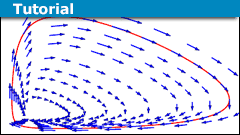
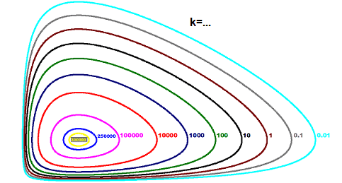
$$
Although we still do not know what $x(t),y(t)$ look like, we already can conclude a few properties of the system. If we vary the constant $k$ and plot the graph of $F(x,y)$, then we get the phase plot or phase space plot of the Lotka-Volterra system,

The three-dimensional graph of $F(x,y)$ looks a bit like a bowl [28].

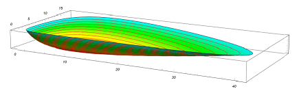
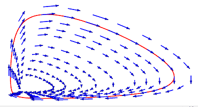
It consists of all possible flows $F(x,y)=1/k$

through the vector field of the differential equation system

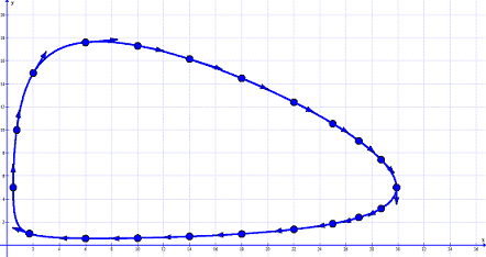
The diagrams show us that

1. None of the two populations can become extinct.
2. Both population sizes vary periodically by time since the flows are closed curves. We already expected this from the informal description.
3. Which flow of all possible ones is the actual one depends only on the initial values of the system, e.g. the red line through the vector field.
4. There must be a critical point at some large value of $k.$
   \begin{align*}
   F_x=\dfrac{\partial F}{\partial x}&=\left(\dfrac{1\cdot e^x}{x^7}-7\dfrac{e^x}{x^8}\right)\cdot \dfrac{e^{2y}}{y^{10}}=\dfrac{(1\cdot x- 7)e^x}{x^8}\cdot \dfrac{e^{2y}}{y^{10}}\\
   F_y=\dfrac{\partial F}{\partial y}&=\left(\dfrac{2\cdot e^{2y}}{y^{10}}-10\dfrac{e^{2y}}{y^{11}}\right)\cdot \dfrac{e^{x}}{x^{7}}=\dfrac{(2\cdot y- 10)e^{2y}}{y^{11}}\cdot \dfrac{e^{x}}{x^{7}}\\[6pt]
   F_x=0 &\Longleftrightarrow x_0=\dfrac{\gamma }{\delta }=7 \\
   F_y=0 &\Longleftrightarrow y_0=\dfrac{\alpha}{\beta}=5
   \end{align*}
   We have therefore a critical point at $(7,5)$ which is a local minimum. It corresponds to $k\approx 332,951$ and $C\approx 12.7.$
5. Assume that $T$ is the common period of both populations. Then
   \begin{align*}
   0&=\log x(T) -\log x(0)=\int_0^T \dfrac{d}{dt}(\log x(t))\,dt=\int_0^T (\alpha – \beta \cdot y(t))\,dt\\&=\alpha T-\beta\int_0^Ty(t)\,dt =10-2\int_0^Ty(t)\,dt
   \end{align*}
   and the mean population size of predators is
   $$
   MV(y) = \dfrac{1}{T}\int_0^T y(t)\,dt = \dfrac{\alpha}{\beta}=5=y_0
   $$
   and analog for the mean population size of prey
   $$
   MV(x) = \dfrac{1}{T}\int_0^T x(t)\,dt = \dfrac{\gamma }{\delta }=7=x_0
   $$
   The mean population sizes of predator and prey are only dependent on the critical point. They are especially independent of the initial values of the system, i.e. equal for any specific solution aka flow.
6. The periodic population sizes are irregular in the sense that we only get pure sines and cosines if the flows are elliptic or a circle.
   \end{enumerate}
   We have thus learned a lot about the situation without actually solving it. This can be done numerically by linearization, i.e. working with small differences instead of differentials. The result [29] in our case is by the Runge-Kutta-Fehlberg method
   

Attractors, Repellers, and Strange Attractors

We have seen that vector fields, like $(F_x,F_y)$ above, are good possibilities for analyzing differential equation systems. We can draw them relatively easily as linear, i.e. first-order approximations and they tell us the course of flows, i.e. solutions. Two phenomena are especially of interest: attractors and repellers. 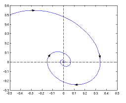An attractor is a region where a flow cannot escape from once it is within, $F(t,A)\subseteq A.$ If an attractor is a point [31], then flows converge to such a point.

A repeller is a negative attractor, a region or point where flows run away from. Switching the directions of the vectors that form an attractor generates a repeller. A magnetic field with its field lines is a good imagination of what attractors and repellers are. Of course, complex vector fields can have both of them and more than one, too. A charged particle is attracted from one side of a dipole and repelled from the other.

 

Edward Norton Lorentz, a US-American meteorologist, and mathematician investigated an idealistic hydrodynamic system to predict states of the atmosphere and found 1963 a strange-looking attractor [32] of
\begin{align*}
\dot X&=a(Y-X)\\
\dot Y&=X(b-Z)-Y\\
\dot Z&=XY-cZ\,.
\end{align*}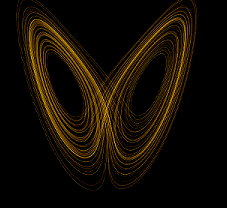
We therefore speak of strange attractors and the one above is the Lorenz attractor. Other famous, and strange attractors are the (Otto) Rössler attractor (1976) [33]
\begin{align*}
\dot X&=-Y-Z\\
\dot Y&=X+aY\\
\dot Z&=b+XZ-cZ\,.
\end{align*}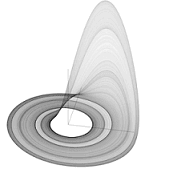
or the (Michel) Hénon attractor for the discrete system
$$
x_{k+1}=y_{k}+1-ax_{k}^{2}\; , \;y_{k+1}=bx_{k}\,.
$$

Theorem of Picard-Lindelöf

We consider a function (flow) on a compact (time) interval $I\subseteq \mathbb{R}$
$$
u\, : \,[a,b] \longmapsto \mathbb{R}^n
$$
and the initial value problem (IVP)
\begin{align*}
\dot{u}(t)=f(t,u(t))\; , \;u(a)=y_0 \qquad ({}^*)
\end{align*}
for a function $f\, : \,[a,b]\times \mathbb{R}^n\longmapsto \mathbb{R}^n$ and ask for solutions. The (global version) of the theorem of Picard-Lindelöf (1890) says, that if $f$ is continuous, and globally Lipschitz-continuous in the second variable, then there exists a unique differentiable solution $\overline{u}$ of the IVP $({}^*)$ for every $y_0\in \mathbb{R}^n,$ and the sequence
$$
v_{k+1}:=y_0 +\int_a^t f(s,v_k(s))\,ds\qquad\qquad t\in [a,b]\, , \,k\in \mathbb{N}_0
$$
converges uniformly to $\overline{u}.$

The idea of the proof is to consider the fixed point equation
$$
u(t)=T.u(t)=u_0+\int_a^t f(s,u(s))\,ds
$$
and prove with the help of the Lipschitz continuity that for the integral operator $T$ holds
$$
\|T.u-T.v\|_\infty \leq L\cdot (b-a)\cdot \|u-v\|_\infty \,,
$$
change to a weighted norm
$$
\|u\|\leq \|u\|_\infty \leq \|u\|e^{\alpha (b-a)}\,,
$$
then prove that we get pointwise
$$
\left|T.u(t)-T.v(t)\right|\leq \dfrac{b-a}{\alpha} \cdot \|u-v\|\cdot e^{\alpha |t-a|}\,,
$$
which means for a suitable choice of $\alpha$ that
$$
\|T.u-T.v\|\leq \dfrac{b-a}{\alpha} \cdot \|u-v\| <\|u-v\|\,.
$$
This means that $T$ is a contraction and the result follows by the Banach fixed-point theorem.$\qquad\;\;\;\;\Box$

It is obvious that the global Lipschitz condition in the second variable, i.e. the flow and solution curve is essential for the theorem. Although the theorem is still applicable to large classes of problems, e.g. the linear case for continuous functions
\begin{align*}
\dot{u}&=A(t)\cdot u + r(t)\\[6pt]
|f(t,u)-f(t,v)|&\leq\displaystyle{\sup_{t\in[a,b]}}|A(t)| \cdot|u-v|\,,
\end{align*}
it is at the same time its greatest weakness. We can prove a local version of the theorem or similar local statements like the theorem of Peano with different conditions, but we cannot eliminate the basic problem to keep the possible flows under control without assuming appropriate conditions beforehand. This is in my opinion system immanent and one of the reasons why Navier-Stokes has made it a Millenium Prize Problem.

We still do not have a satisfactory answer as to whether there are undoubtedly hard problems in this world or whether we simply failed to find smart solutions.

Sources