Computing the Riemann Zeta Function Using Fourier Series
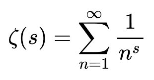
Table of Contents
Euler’s amazing identity
The mathematician Leonard Euler developed some surprising mathematical formulas involving the number ##\pi##. The most famous equation is ##e^{i \pi} = -1##, which is one of the most important equations in modern mathematics, but unfortunately, it wasn’t invented by Euler.Something that is original with Euler is this amazing identity:
Equation 1: ##1 + 1/4 + 1/9 + 1/16 + … = \pi^2/6##
This is one instance of an important function called the Riemann Zeta function, ##zeta(s)##, which in the case where ##s > 1## is defined by:
Equation 2: ##\zeta(s) = \sum_{j=1}^\infty \dfrac{1}{j^s}##
So Euler’s identity can be written as:
Equation 3: ##\zeta(2) = \frac{\pi^2}{6}##
This post is an attempt to show how you can derive that result, and related results, using facts about trigonometry, complex numbers, and the Fourier series.
Some related functions defined via Fourier series
I’m not a mathematician, but a physicist by training, so how would I go about proving Euler’s second equation? How would I evaluate ##\zeta(s)## for other values of ##s##?
Well, my inclination, having lots of experience with the Fourier series, would be to make the following definitions:
Equation 4: ##S_n(x) = \sum_{j=1}^\infty \dfrac{sin(jx)}{j^n}##
Equation 5: ##C_n(x) = \sum_{j=1}^\infty \dfrac{cos(jx)}{j^n}##
Then to get ##\zeta(n)##, note that it is equal to ##C_n(0)##. So how do we compute those functions?
Let’s look at the very first one,
Equation 6: ##C_0(x) = \sum_{j=1}^\infty cos(jx)##
What function is that? Clearly, when ##x = 0##, then ##C_0(0) = \infty##. So it’s not very well-behaved, but physicists aren’t frightened by such things. Can we evaluate this when ##x \neq 0##? Yes, in a physicists hand-wavy sense.
Detour: The Fourier representation of the Delta function (which isn’t actually a function)
Let’s look at a related sum:
Equation 7: ##F(x) = \sum_{j=-\infty}^\infty e^{i j x}##
This is related in a simple way to ##C_0(x)##, because we can use ##e^{i j x} = cos(jx) + i sin(jx)##. We can break up and rearrange the infinite sum to take advantage of this:
##F(x) = \sum_{j=-\infty}^\infty e^{i j x} = \sum_{j= -\infty}^{-1} e^{i j x} + 1 + \sum_{j= 1}^{\infty} e^{i j x} = \sum_{j= 1}^{\infty} e^{-i j x} + 1 + \sum_{j= 1}^{\infty} e^{i j x} = 1 + 2\sum_{j= 1}^{\infty} cos( j x) ##
So if we knew ##F(x)##, we could compute ##C_0(x)##, via:
Equation 8: ##C_0(x) = \frac{1}{2} F(x) + \frac{1}{2}##
Evaluating the infinite sum using a famous summation trick
So what is ##F(x)##? Well, when ##x=0##, we have ##\sum_{j=-\infty}^{+\infty} 1 = \infty##. So we conclude
Equation 9: ##F(0) = \infty##
It’s equal to ##\infty## when ##x=0##, but maybe it converges to something when ##x \neq 0##? We can evaluate it, under the assumption that the summation converges, by using a standard summation trick:
##u + u^2 + u^3 + … = \dfrac{u}{1-u}##
(IF you don’t know this trick, you can prove it to yourself by letting ##S = u + u^2 + u^3 + … ##, then multiplying both sides by ##u## gives ##uS = u^2 + u^3 + u^4 + …
= S – u##. So ##S## satisfies the equation: ##uS = S – u##. Algebra gives ##S = \dfrac{u}{1-u}##.)
We can use this trick on our series defining ##F(x)## (after splitting positive and neg
##F(x) = \sum_{j= -\infty}^{\infty} e^{-i j x} = \sum_{j= 1}^{\infty} e^{-i j x} + 1 + \sum_{j= 1}^{\infty} e^{i j x}##
In the first summation, we can let ##u = e^{-ix}## to get
Sum 1 = ##\sum_{j= 1}^{\infty} e^{-i j x} = \dfrac{e^{-ix}}{1 – e^{-ix}}##
similarly, the second summation gives:
Sum 2 = ##\sum_{j= 1}^{\infty} e^{i j x} = \dfrac{e^{ix}}{1 – e^{ix}}##
We can make Sum 2 have the same denominator as Sum 1 by multiplying top and bottom by ##- e^{-ix}##:
Sum 2 = ##\dfrac{e^{ix}}{1 – e^{ix}} = \dfrac{e^{ix} \cdot -e^{ix}}{(1 – e^{ix}) \cdot -e^{-ix}} = \dfrac{-1}{1 – e^{-ix}}##
So we can rewrite ##F(x)## as follows:
##F(x) = ##Sum 1 + Sum 2 + 1 ## = \dfrac{e^{-ix}}{1 – e^{-ix}} + \dfrac{-1}{1 – e^{-ix}} + 1= \dfrac{e^{-ix} – 1}{1 – e^{-ix}} + 1 = -1 + 1 = 0##
Equation 10: ##F(x) = 0## when ##x \neq 0##
Integral property of ##F(x)##
So we find that our ##F(x)## is infinite when ##x=0## and when ##x \neq 0## it’s equal to 0. So it’s a pretty weird function, but we can establish something else about ##F(x)##. Let’s for the hell of it integrate ##F(x)##:
##\int_{- \pi}^{+\pi} F(x) dx = \int_{- \pi}^{+\pi} (\sum_{j=-\infty}^{+\infty} e^{ijx}) dx##
Since we just established that ##F(x) = 0## for any ##x \neq 0## (actually, for any ##x## such that the summation converges), we know that this integral should be zero. On the other hand, if we could swap the summation and the integration, we would have something very different:
##\int_{- \pi}^{+\pi} F(x) dx = \sum_{j=-\infty}^{+\infty} \int_{- \pi}^{+\pi} e^{ijx} dx##
The integral ## \int_{- \pi}^{+\pi} e^{ijx} dx## just gives 0 unless ##j=0##, in which case it gives ##2\pi##. So we get the fact:
Equation 11: ##\int_{- \pi}^{+\pi} F(x) dx = 2 \pi##
Introducing the delta function
The Dirac delta function is a mythical beast (not a real function) with the following properties
- ##\delta(0) = \infty##
- ##\delta(x) = 0## (when ##x \neq 0##)
- ##\int \delta(x) dx = 1## (when the region of integration includes ##x=0##)
Comparing this to what we proved about ##F(x)## (or handwaved, actually), we discover
Equation 12: ##F(x) = 2 \pi \delta(x)##
First comment
As I said, there is no actual function satisfying these properties, because any function that is zero except at one point integrates to 0. So how does it make any sense to say the following?
##F(x) = \sum_{j=-\infty}^{+\infty} e^{ijx} = 2 \pi \delta(x)##
Well, there’s a physicist’s way of making sense of it, which is to understand the summation as being a finite sum and then taking the limit at the end. If we modify ##F(x)## by letting ##F_N(x) = \sum_{j=-N}^{+N} e^{ijx}##, then we have, for any smooth function ##f(x)##,
##lim_{N \rightarrow \infty} \int f(x) F_N(x) dx = f(0)## (if the region of integration includes ##x=0##
##lim_{N \rightarrow \infty} \int f(x) F_N(x) dx = 0## (if the region of integration does not include ##x=0##
Second comment
Since ##F(x)## is defined in terms of ##e^{ijx}##, we automatically know that ##F(x)## is periodic: ##F(x+2n\pi) = F(x)##. Therefore, strictly speaking, we should write:
##F(x) = 2 \pi \sum_{n=-\infty}^{+\infty} \delta(x – 2n \pi)##
I’m not going to talk any more about how one can rigorously deal with these not-quite-functions (called “distributions”), but I just want to let you know that there’s a lot of subtlety involved in making sense of it all.
Evaluating ##C_0(x)## and ##S_1(x)##
Okay, now we’re ready to get back to the functions I defined earlier:
##S_n(x) = \sum_{j=1}^{\infty} \dfrac{sin(jx)}{j^n}##
##C_n(x) = \sum_{j=1}^{\infty} \dfrac{cos(jx)}{j^n}##
When ##n=0##, we have ##C_0(x) = \sum_1^{\infty} cos(jx)##. Since the cosine can be written in terms of exponentials, we can rewrite this as:
##C_0(x) = \sum_1^{\infty} \dfrac{e^{i j x} + e^{-i j x}}{2}##
That summation is almost the same as ##\frac{1}{2} \sum_{-\infty}^{\infty} e^{i j x}##, except the expression for ##C_0(x)## is missing the ##j=0## term, which is just equal to ##\frac{1}{2}##. So we can conclude:
##C_0(x) = \frac{1}{2} (F(x) – 1)##
Using the fact that ##F(x)## is a representation of ##2 \pi \delta(x)##, we have:
Equation 13: ##C_0(x) = \pi \delta(x) – \frac{1}{2}##
Now, to get ##S_1(x)##, just integrate the left-hand side (once again, doing a (dubious) exchange of summation and integration):
##\int_{-x}^{+x} C_0(x) dx = \int_{-x}^{+x} \sum_{j=1}^{\infty} cos(jx) dx = = \sum_{j=1}^{\infty} \int_{-x}^{+x} cos(jx) dx = \sum_{j=1}^{\infty} \dfrac{2 sin(jx)}{j} = 2 S_1(x)##
So we conclude:
Equation 14: ##S_1(x) = \dfrac{1}{2} \int_{-x}^{+x} C_0(x) dx##
So that’s what we get when we integrate the left-hand side of Equation 14. Integrating the right-hand side is a tiny bit subtle:
If ##x > 0##, then ##\int_{-x}^{+x} \delta(x) dx = +1##. If ##x < 0##, then you have to get the opposite sign, because symmetrically integrating an even function has to produce an odd function, so when ##x < 0##, ##\int_{-x}^{+x} \delta(x) dx = -1##. We can put those two facts together by introducing the “sign” function,
##\text{sign}(x) = -1## if ##x < 0##
##= 0## if ##x = 0##
##= +1## if ##x > 0##
Then
Equation 15: ##\int_{-x}^{+x} \delta(x) dx = \text{sign}(x)##.
Using this result, we can evaluate:
##\int_{-x}^{+x} (\pi \delta(x) – \frac{1}{2}) dx = \pi \text{sign}(x) – x##
So we now have an explicit expression for ##S_1(x)##:
##S_1(x) = \sum_{j=1}^{\infty} \dfrac{sin(jx)}{j} = \frac{1}{2} \int_{-x}^{+x} C_0(x) dx = \frac{\pi}{2} \text{sign}(x) – \dfrac{x}{2}##
Equation 16: ##S_1(x) = \frac{\pi}{2} \text{sign}(x) – \dfrac{x}{2}##
Note:
The above expression for ##S_1(x)## only is valid in the region ##-\pi < x < \pi##. To get its value for other choices of ##x##, you have to use the fact that it is periodic: ##S_1(x+2 \pi) = S_1(x)##.
Alternative derivation that doesn’t use delta-functions
Our infinite series for ##C_0(x)## doesn’t actually converge to an honest-to-god function. The series for ##S_1(x)## does converge though. So we should be able to prove the identity without using the dubious delta-function. We can do that. Since ##e^{ijx} = cos(jx) + i sin(jx)##, we can write:
##\sum_{j=1}^{\infty} \dfrac{sin(jx)}{j} = \text{Im}(\sum_{j=1}^{\infty} \dfrac{e^{ijx}}{j})##
##\sum_{j=1}^{\infty} \dfrac{cos(jx)}{j} = \text{Re}(\sum_{j=1}^{\infty} \dfrac{e^{ijx}}{j})##
where ##\text{Im}## means “take the imaginary part”, and ##\text{Re}## means take the real part, provided that the right-hand side converges, which it does whenever ##x## is unequal to ##0##, ##2\pi##, etc. To evaluate the right-hand side, we can use another summation trick:
##\sum_{j=1}^{\infty} \dfrac{u^j}{j} = \text{log}(\dfrac{1}{1-u})##
We can substitute ##u = e^{ix}## to get:
Equation 17: ##S_1(x) = \text{Im}(\text{log}(\dfrac{1}{1 – e^{ix}}))##
Equation 17b: ##C_1(x) = \text{Re}(\text{log}(\dfrac{1}{1 – e^{ix}}))##
##\dfrac{1}{1 – e^{ix}}## is not a convenient form for taking logarithms. What we would like is to write the expression as ##R e^{i \theta}## where ##R## is a positive real. Then the logarithm is given by: ##\text{log}(R e^{i \theta}) = log(R) + i \theta##. Then it’s easy to take the imaginary part. But we have to massage the actual term into this form.
If you want to skip to the punch line, it’s this:
Equation 18: ##\dfrac{1}{1 – e^{ix}} = \dfrac{e^{-i x/2 \pm \pi/2}}{2 |sin(\dfrac{x}{2})|}##
where in the exponent, you choose ##+\frac{\pi}{2}## if ##sin(\dfrac{x}{2}) > 0## and ##-\frac{\pi}{2}## otherwise.
Taking the logarithm of both sides gives:
Equation 19: ##log(\dfrac{1}{1 – e^{ix}}) = -i \frac{x}{2} \pm i \frac{\pi}{2} – log(2 |sin(\dfrac{x}{2})|)##
According to Equation 17, we get ##S_1(x)## by taking the imaginary part of this. So we get
Equation 20: ##S_1(x) = – \frac{x}{2} \pm \frac{\pi}{2} = -\frac{x}{2} + sign(x) \frac{\pi}{2}##
So this gives Equation 16: in a different way, without detouring through delta functions.
Taking the real part of Equation 19: gives as ##C_1(x)##:
Equation 20b: ##C_1(x) = – log(2 |sin(\dfrac{x}{2})|)##
The gory details
The details depend on facts about trigonometry and exponentiation.
We can write: ##1 – e^{ix} = 1 – (cos(x) + i sin(x)) = (1-cos(x)) + i sin(x)##. Here we can use a half-angle formula to write: ##1 – cos(x) = 2 sin^2(\dfrac{x}{2})##, and another half-angle formula to write: ##sin(x) = 2 sin(\dfrac{x}{2}) cos(\dfrac{x}{2})##. So we have:
##1 – e^{ix} = 2 sin^2(\dfrac{x}{2}) – 2i sin(\dfrac{x}{2})cos(\dfrac{x}{2}) = 2 sin(\dfrac{x}{2}) (sin(\dfrac{x}{2}) – i cos(\dfrac{x}{2}))##
Another fact about sines and cosines: ##sin(\dfrac{x}{2}) = cos(\dfrac{x}{2} – \dfrac{\pi}{2}))## and ##- cos(\dfrac{x}{2}) = sin(\dfrac{x}{2} – \dfrac{\pi}{2}))##. So we can rewrite this as:
##1 – e^{ix} = 2 sin(\dfrac{x}{2}) (cos(\dfrac{x}{2} – \dfrac{\pi}{2}) + i sin(\dfrac{x}{2} – \dfrac{\pi}{2})) = 2 sin(\dfrac{x}{2}) e^{i x/2 – \pi/2)}##
##= 2 sin(\dfrac{x}{2}) e^{-i \pi/2 + ix/2}##
So if ##x > 0##, we can write this as:
Equation 21: ##1 – e^{ix} = |2 sin(\dfrac{x}{2})| e^{-i \pi/2 + x/2}## (when ##x > 0##)
If ##x## is negative, then we can write: ##sin(\dfrac{x}{2}) = – |sin(\dfrac{x}{2})| = |sin(\dfrac{x}{2})| e^{i \pi}## (since ##-1 = e^{i \pi}##), so
Equation 22: ##1 – e^{ix} = 2 |sin(\dfrac{x}{2})| e^{+i \pi/2 + i x/2}## (when ##x < 0##)
To cover both cases, we can write:
##1 – e^{ix} = 2 |sin(\dfrac{x}{2})| e^{i x/2 \mp i \pi/2}##
where we take ##- \frac{\pi}{2}## when ##x > 0## and ##+ \frac{\pi}{2}## if ##x < 0##.
Taking reciprocals of both sides gives (using ##\dfrac{1}{e^{iu}} = e^{-iu}##)
##\dfrac{1}{1 – e^{ix}} = \dfrac{e^{-i x/2 \pm i \pi/2}}{2 |sin(\dfrac{x}{2})|}##
Which gives us our Equation 18:
Comment
The criterion for choosing the plus sign or minus sign depends on the sign of ##sin(\frac{x}{2})##, not on the sign of ##x##. However, since we will be only considering the case where ##-\pi < x < +\pi##, in this region, ##x## is positive exactly when ##sin(\frac{x}{2})## is positive.
A Cool Fact Provable from ##S_1(x)##
So we have the identity:
Equation 23: ##S_1(x) = \sum_{j=1}^{\infty} \dfrac{sin(jx)}{j} = \frac{-x}{2} + \text{sign}(x) \frac{\pi}{2}##
(As I mentioned earlier, ##S_1(x)## is periodic, so this equation literally only holds in the region ##-\pi < x < +\pi##. To get ##S_1(x)## for some other value of ##x##, just use ##S_1(x) = S_1(x + 2n \pi)##)
Let’s look at some values. First, ##S_1(0) = 0##. That checks out, because ##sin(0) = 0## and so is the right-hand side of Equation 23 (remember ##\text{sign(0)}## is 0).
Second, ##S_1(\pi) = 0##. That’s because ##sin(j\pi) = 0##, and the right-hand side of Equation 23 gives: ##-\pi/2 + \pi/2## (since ##sign(\pi) = +1##).
Third, ##S_1(- \pi) = 0##. That’s because ##sin(-j\pi) = 0##, and the right-hand side of Equation 23 gives: ##+\pi/2 – \pi/2## (since ##sign(-\pi) = -1##).
A more interesting example is ##x = \dfrac{\pi}{2}##. The definition of ##S_1(x)## gives:
##S_1(\pi/2) = \sum_{j=1}^{\infty} \dfrac{sin(j\pi/2)}{j}##
Since ##sin(j\pi/2) = 0## for ##j= 0, \pm 2, \pm 4 …## and ##sin(j\pi/2) = +1## for ##j=1, 5, 9, …## and ##sin(j\pi/2) = -1## for ##j = 3, 7, 11, …##, we can write this as:
##S_1(\pi/2) = \dfrac{1}{1} – \dfrac{1}{3} + \dfrac{1}{5} – \dfrac{1}{7}…##
The right-hand side of the identity Equation 23 gives:
##S_1(\pi/2) = -\dfrac{\pi}{4} + \dfrac{\pi}{2} = +\dfrac{\pi}{4}##
So we conclude:
Equation 24: ##S_1(\pi/2) = \dfrac{1}{1} – \dfrac{1}{3} + \dfrac{1}{5} – \dfrac{1}{7} … = \dfrac{\pi}{4}##
(Note: Equation 24 can also be derived by looking at the power series for ##tan^{-1}(x)## evaluated at ##x = 1##.)
Recurrence relations for ##S_n(x)## and ##C_n(x)##
We’re really close to the goal of showing how to compute the Riemann zeta function ##\zeta(2)## and proving that it’s equal to ##\frac{\pi^2}{6}## as in Equation 1 and Equation 2. We will actually do better than that, by showing how to compute ##\zeta(n)## for any even positive value of ##n##.
Note:
The techniques here don’t tell how to compute exactly ##\zeta(n)## for ##n## odd, and they don’t tell us what to do for ##n < 0##, either. Some negative values of ##n## are exactly computable, but deriving that goes beyond this article.
Looking at the definitions of ##S_n(x)## and ##C_n(x)##, we can see that we can relate ##S_n(x)## and ##C_{n+1}(x)## as follows:
##S_n(x) = \sum_{j=1}^{\infty} \dfrac{sin(jx)}{j^n}##
Now, note that
Equation 25: ##\int_{0}^x sin(jx) dx = 1/j (-cos(jx) ) |_{0}^{x} = (-cos(jx) -(-1))/j = (1-cos(jx))/j##
So if we multiply both sides of Equation 25 by ##1/j^n## and sum, we find:
Equation 26: ##\int_{0}^{x} S_n(x) dx = \sum_{j=1}^\infty \int_{0}^x sin(jx)/j^n dx = \sum_{j=1}^\infty (1-cos(jx))/j^{n+1} = (\sum_{j=1}^\infty 1/j^{n+1}) – (\sum_{j=0}^{\infty}cos(jx)/j^{n+1})##
Which, given our definitions of ##C_{n+1}(x)## and ##\zeta(n+1)##, implies
Equation 27: ##\int_{0}^{x} S_n(x) dx = \zeta(n+1) – C_{n+1}(x)##
A special case, to be used later, is:
Equation 28: ##\int_{0}^{\pi} S_n(x) dx = \zeta(n+1) – C_{n+1}(\pi)##
We can also get an identity for the integral of ##C_n##
Equation 29: ##\int_{0}^{x} C_n(x) dx = \sum_{j=1}^\infty \int_{0}^x cos(jx)/j^n dx = \sum_{j=1}^\infty sin(jx)/j^{n+1}##
So we have:
Equation 30: ##\int_{0}^{x} C_n(x) dx = S_{n+1}(x)##
So as long as ##S_n(x)## and ##C_n(x)## are simple functions, then we can integrate to get ##C_{n+1}## and ##S_{n+1}##. Except for one thing: Equation 27 only gives us ##C_{n+1}(x)## if we already know ##\zeta(n+1)##, which is exactly what we’re trying to find.
But, there is yet another trick up our sleeves. Let’s look at ##C_n(\pi)##. By the definition of ##C_n##, this is given by:
Equation 31: ##C_n(\pi) = \sum_{j=1}^{\infty} cos(j\pi)/j^n##
Since ##cos(j\pi) = -1## for ##j## odd, and ##cos(j\pi) = 1## for ##j## even, this means:
Equation 32: ##C_n(\pi) = \sum_{j=1}^{\infty} (-1)^{j}/j^n##
That’s almost ##\zeta(n)##, except that the terms are alternating sign in ##C_n(\pi)## while they are all positive in ##\zeta(n)##. But if we add the two together, the odd entries will cancel:
##C_n(\pi) + \zeta(n) = 2 \sum’_j 1/j^n## where the ##’## means that the sum is only over positive even values of ##j##. We can change indices by letting ##j = 2k## to get:
##C_n(\pi) + \zeta(n) = 2\sum_{k=1}^\infty 1/(2k)^n = 2/2^n \sum_{k=1}^\infty 1/k^n = 2/2^n \zeta(n)##
Rearranging, we get:
Equation 33: ##C_n(\pi) = – (1 – 2/2^n) \zeta(n)##
Okay, so using Equation 33 together with Equation 28 gives us:
##\int_{0}^{\pi} S_n(x) dx = \zeta(n+1) – C_{n+1}(\pi) = \zeta(n+1) + (1 – 2/2^{n+1}) \zeta(n+1)##. So rearranging gives us an identity for ##\zeta(n+1)##:
Equation 34: ##\zeta(n+1) = \dfrac{2^n}{2^{n+1} – 1} \int_{0}^{\pi} S_n(x) dx##.
Summary of the Recurrence Relations
Just to have them in one place, here are the recurrence relations that allow you to compute ##C_n(x)## and ##zeta(n)## for even ##n## and ##S_n(x)## for odd ##n##:
- ##S_1(x) = -\dfrac{x}{2} + sign(x) \dfrac{\pi}{2}## (This allows us to compute ##S_1(x)##)
- ##\zeta_{n+1}(x) =\dfrac{2^n}{2^{n+1} – 1} \int_{0}^{\pi} S_n(x) dx## (This allows us to compute ##\zeta(2)##)
- ##C_{n+1}(x) = \zeta(n+1) – \int_{0}^{x} S_n(x) dx## (This allows us to compute ##C_2(x)##)
- ##S_{n+1}(x) = \int_{0}^{x} C_n(x) dx## (This allows us to compute ##S_3(x)##. Then we can return to equation 2 to compute ##\zeta(4)##. Etc.)
These facts give us (with some trivial integration) ##\zeta(n)## for all positive even ##n##.
Finally, Euler’s Identity
By recurrence equation 1. above, we have ##S_1(x) = -\dfrac{x}{2} + sign(x) \dfrac{\pi}{2}##. Integrate from 0 to ##\pi##:
##\int_{0}^\pi S_1(x) = -\pi^2/4 + \pi^2/2 = \pi^2/4##
By recurrence equation 2. above, we have:
Equation 35: ##\zeta(2) = \dfrac{2}{2^{2} – 1} \pi^2/4 = 2/3 * \pi^2/4 = \pi^2/6##
The next values of ##S_n, C_n, \zeta_n##
Using recurrence relation 3., we can compute ##C_2(x)## from ##S_1(x)##:
##C_2(x) = \zeta(s) – \int_0^{x} S_1(x) dx = \pi^2/6 – \int_0^{x} (-x/2 + sign(x) \pi/2)dx = (\pi^2/6) + (1/4) x^2 – (sign(x) \pi/2) x##
Then using recurrence relation 4., we can compute ##S_3(x)## from ##C_2(x)##:
##S_3(x) = \int_0^x C_2(x) dx = (\pi^2/6) x + (1/12) x^3 – (sign(x) \pi/4) x^2##
Then we can use recurrence relation 2. to compute ##\zeta(4)##:
##\zeta(4) = \dfrac{2^3}{2^{4} – 1} \int_0^\pi S_3(x) dx = 8/15 (\pi^4/12 + \pi^4/48 – \pi^4/12) = 8/15 \cdot \pi^4/48 = \pi^4/90##
Some plots
It’s nice to have some graphics to break up a boring article of text and mathematics. So here are some plots of functions mentioned. I used an online function plotting app, available here:
FOOPLOT
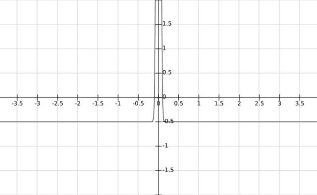
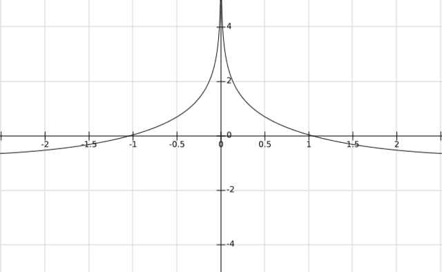
##C_0(x)##
This function is ##\pi \delta(x) – 1/2##. Since you can’t actually plot the delta function, since it’s not a real function, I’m using a stand-in. The function ##f(x) = \sqrt{\lambda/\pi} e^{-\lambda x^2}## works sort of like a delta function when ##\lambda## is large, because
- ##f(0) = \sqrt{\lambda/\pi} \rightarrow \infty## as ##\lambda \rightarrow \infty##
- ##f(x) \rightarrow 0## as ##\lambda \rightarrow \infty##, if ##|x| \gt 0##
- ##\int_{-\infty}^{+\infty} f(x) dx = 1##
So as a stand-in for the delta function, I used that function ##f(x)## with ##\lambda = 400##. The result:
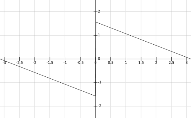
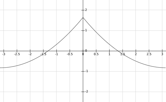
##S_1(x)##
This is the function ##S_1(x) = -\frac{x}{2} + sign(x) \frac{\pi}{2}##
##C_1(x)##
This is the function ##C_1(x) = -log(2 |sin(x/2)|)##
##C_2(x)##
This is the function ##C_2(x) = (\pi^2/6) + (1/4) x^2 – (sign(x) \pi/2) x##
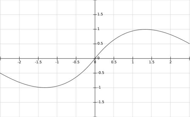
##S_3(x)##
This is the function ##S_3(x) = \int_0^x C_2(x) dx = (\pi^2/6) x + (1/12) x^3 – (sign(x) \pi/4) x^2##
Going Further
The techniques described here can give you ##S_n(x)## for odd values of ##n## and ##\zeta(n)## and ##C_n(x)## for even values of ##n##. Going further along these lines is not very productive. Looking back at Equation 20b, we can see an expression for ##C_1(x)##:
##C_1(x) = -log(2 |sin(x/2)|)##
To get to ##S_2(x), \zeta(3), C_3(x), …## via our recursion relations, we have to be able to integrate that expression, which is not one of the integrals that I know how to do. We could certainly integrate numerically, but it’s not clear if that would be better than just numerically summing the series expressions.
Recurrence relations involving the coefficients
As you can see, there is a definite pattern in going from ##S_1(x)## to ##C_2(x)## to ##S_3(x)##, etc. At each stage, you get a polynomial in ##x## (ignoring the ##sign(x)## function, which always gives +1 if we’re considering ##x > 0##).
##S_1(x) = s_{1,0} + s_{1,1} x##
##C_2(x) = c_{2,0} + c_{2,1} x + c_{2,2} x^2##
##S_3(x) = s_{3,1} x + s_{3,2} x^2 + s_{3,3} x^3##
and in general,
##S_n(x) = s_{n,1} x + s_{n,2} x^2 + … + s_{n,n} x^n##
##C_n(x) = c_{n,0} + c_{n,2} x + … + c_{n,n} x^n##
Then ##\zeta(n) = c_{n,0}##
So rather than doing lots of integrals, we could look for a pattern involving the coefficients ##c_{i,j}## and ##s_{ij}##. I’m not going to pursue this, but I hear that it involves the Bernoulli numbers, which come up in lots of areas of number theory and Fourier analysis, and differential equations.
What about ##\zeta(n)## when ##n## is negative? Or a fraction?
The other big area to explore with the Riemann zeta function is ##zeta(n)## when ##n## is negative. That seems to be nonsensical, because the definition of ##\zeta(n)## is:
##\sum_{j=1}^\infty \frac{1}{j^n}##
If we let ##n## be negative, then it means that the terms in the summation get bigger and bigger. For example, for ##n=-1##, we would have:
##\sum_{j=1}^\infty \frac{1}{j^{-1}} = \sum_{j=1}^\infty j = 1 + 2 + 3 + …##
That surely adds up to infinity, right? No, that summation doesn’t converge. However, it is possible to define ##\zeta(s)## in a way that makes sense for every value of ##s## (except ##s=1##) and which happens to be equal to ##\sum \frac{1}{j^s}## when ##s > 0##. To develop ##\zeta(s)## for negative values of ##s##, it turns out that Fourier series are again going to be useful. But that’s a different post…


”
I’ve checked chrome and safari and your link is broken in both. There appears to be garbage prior to the working URL. Is this the correct one?
”
Yes. I have extended the results in that insight and I will update it Really Soon Now (as Jerry Pournelle used to say).
”
Did you check out my Insight on this
”
I’ve checked chrome and safari and your link is broken in both. There appears to be garbage prior to the working URL. Is this the correct one?
[URL=’https://www.physicsforums.com/insights/explore-the-fascinating-sums-of-odd-powers-of-1-n/’]Explore the Fascinating Sums of Odd Powers of 1/n Source https://www.physicsforums.com/insights/explore-the-fascinating-sums-of-odd-powers-of-1-n/%5B/URL%5D
So we can define a number of functions related to the zeta-function:
##\zeta(s) = \sum j^{-s}##
The odd zeta function:
##O(s) = ## the sum restricted to even values of ##j##
##= \sum_j (2j + 1)^{-s}##
The alternating zeta function:
##A\zeta(s) = \sum j^{-s} (-1)^j##
The alternating odd zeta function:
##AO(s) = \sum {2j+1}^{-s} (-1)^j##
”
Did you check out my Insight on this ([URL=’http://Explore the Fascinating Sums of Odd Powers of 1/n Source https://www.physicsforums.com/insights/explore-the-fascinating-sums-of-odd-powers-of-1-n/'%5DExplore the Fascinating Sums of Odd Powers of 1/n Source https://www.physicsforums.com/insights/explore-the-fascinating-sums-of-odd-powers-of-1-n/%5B/URL%5D )? You will also find references to two earlier Insights, one of which shows how to calculate the Zeta function for all even values of s.
”
No, I had not read those. Thanks!
Did you check out my Insight on this ([URL=’http://Explore the Fascinating Sums of Odd Powers of 1/n Source https://www.physicsforums.com/insights/explore-the-fascinating-sums-of-odd-powers-of-1-n/'%5DExplore the Fascinating Sums of Odd Powers of 1/n Source https://www.physicsforums.com/insights/explore-the-fascinating-sums-of-odd-powers-of-1-n/%5B/URL%5D )? You will also find references to two earlier Insights, one of which shows how to calculate the Zeta function for all even values of s.