Higher Prequantum Geometry II: The Principle of Extremal Action – Comonadically

 

 

The previous article motivated the importance of considering “pre-quantum field theory” in-between classical and quantum field theory. This article here reviews modern classical field theory from a perspective that will be useful for this purpose.

Most field theories of relevance in theory and in nature are local Lagrangian field theories (and those that do not tend to be holographic boundary theories of those that are). This means that their equations of motion are partial differential equations obtained as Euler-Lagrange equations of a local variational principle. This is the modern incarnation of the time-honored principle of extreme action.

We review here how this is formalized, from a category-theoretic point of view that will point the way to prequantum field theory.

This article is indebted to discussion with Igor Khavkine.

---

 

The kinematics of a field theory is specified by a smooth manifold $\Sigma$ of dimension $(p+1)$ and a smooth bundle $E$ over $\Sigma$. A field configuration is a smooth section of $E$. If we think of $\Sigma$ as being spacetime, then typical examples of fields are the electromagnetic field or the field of gravity. But we may also think of $\Sigma$ as being the worldvolume of a particle (such as the electron in the previous article) or of a higher dimensional “brane” that propagates in a fixed background of such spacetime fields, in which case the fields are the maps that encode a given trajectory.

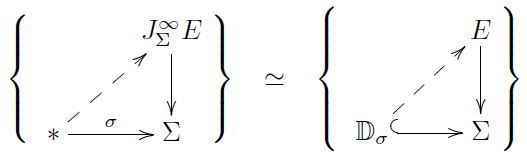
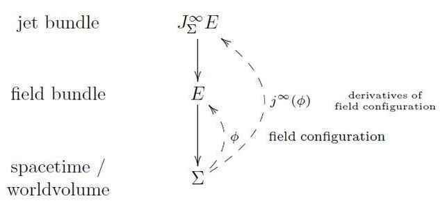
The dynamics of a field theory are specified by an equation of motion, a partial differential equation for such sections. Since differential equations are equations among all the derivatives of such sections, we consider the spaces that these form: the jet bundle $J^\infty_\Sigma E$ is the bundle over $\Sigma$ whose fiber over a point $\sigma \in \Sigma$ is the space of sections of $E$ over the infinitesimal neighborhood $\mathbb{D}_\sigma$ of that point:

Therefore every section $\phi$ of $E$ yields a section $j^\infty(\phi)$ of the jet bundle, given by $\phi$ and all its higher order derivatives.

Accordingly, for $E, F$ any two smooth bundles over $\Sigma$, then a bundle map,

 

encodes a (non-linear) differential operator $D_f : \Gamma_\Sigma(E) \longrightarrow \Gamma_\Sigma(F)$ by sending any section $\phi$ of $E$ to the section $f \circ j^\infty(\phi)$ of $F$. Under this identification, the composition of differential operators $D_g \circ D_f$ corresponds to the “Kleisli-composite” of $f$ and $g$, which is

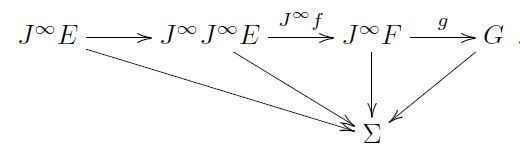
Here the first map is given by re-shuffling derivatives and gives the jet bundle construction $J^\infty_\Sigma$ the structure of a co-monad — the jet comonad.

Differential operators are so ubiquitous in the present context that it is convenient to leave them notationally implicit and understand every morphism of bundles $E \longrightarrow F$ to designate a differential operator $D : \Gamma_\Sigma(E)\longrightarrow \Gamma_\Sigma(F)$. This is what we will do from now on. Mathematically this means that we are now in the co-Kleisli category $\mathrm{Kl}(J^\infty_\Sigma)$ of the jet comonad
$$
\mathrm{DiffOp}_\Sigma \simeq \mathrm{Kl}(J^\infty_\Sigma)
\,.
$$

For example the de Rham differential is a differential operator from sections of $\wedge^{p}T^\ast \Sigma$ to sections of $\wedge^{p+1}T^\ast \Sigma$ and hence now appears as a morphism of the form
$$
d_H : \wedge^{p}T^\ast \Sigma \longrightarrow \wedge^{p+1}T^\ast \Sigma
\,.
$$
With this notation, a globally defined local Lagrangian for fields that are sections of some bundle $E$ over spacetime/worldvolume $\Sigma$ is simply a morphism of the form
$$
L : E \longrightarrow \wedge^{p+1}T^\ast \Sigma
\,.
$$
Unwinding what this means, this is a function that at each point of $\Sigma$ sends the value of field configurations and all their spacetime/worldvolume derivatives at that point to a $(p+1)$-form on $\Sigma$ at that point. It is this pointwise local (in fact: infinitesimally local) dependence that the term local in local Lagrangian refers to.

Notice that this means that $\wedge^{p+1} T^\ast \Sigma$ serves the role of the moduli space of horizontal $(p+1)$-forms, in that horizontal $(p+1)$-forms on $J^\infty_\Sigma E$ are now identified with morphisms from $E$ into this object $\wedge^{p+1}T^\ast \Sigma$:
$$
\Omega^{p+1}_H(E) = \mathrm{Hom}_{\mathrm{DiffOp}_\Sigma}(E,\wedge^{p+1}T^\ast \Sigma)
\,.
$$

Regarding such $L$ for a moment as just a differential form on $J^\infty_\Sigma(E)$, we may apply the de Rham differential $d$ on $J^\infty \Sigma E$ to it. One finds that this uniquely decomposes as a sum of the form

$$
d L = \mathrm{EL} – d_H \Theta
\,.
$$

for some $\Theta$ and for $\mathrm{EL}$ pointwise the pullback of a vertical 1-form on $E$; such a differential form is called a source form:

$$
\mathrm{EL} \in \Omega^{p+1,1}_S(E)
\,.
$$

This particular source form is of paramount importance: the equation
$$
\underset{v\in \Gamma(V E)}{\forall} j^\infty(\phi)^\ast \iota_v\mathrm{EL} = 0
$$
on sections $\phi \in \Gamma_\Sigma(E)$ is a partial differential equation, and this is called the Euler-Lagrange equation of motion induced by $L$. Differential equations arising this way from a local Lagrangian are called variational.

A little reflection reveals that this is indeed a re-statement of the traditional prescription of obtaining the Euler-Lagrange equations by locally varying the integral over the Lagrangian and then applying partial integration to turn all variation of derivatives (i.e. of jets) of fields into a variation of the fields themselves. Here we do not consider this under the integral, and hence the boundary terms arising from the would-be partial integration show up as the contribution $\Theta$.

We step back to say this more neatly. In general, a differential equation on sections of a bundle $E$ is what characterizes the kernel of a differential operator. Now such kernels do not, in general, exist in the Kleisli category $\mathrm{DiffOp}_\Sigma$ of the jet comonad that we have been using, but (as long as it is non-singular) it does exist in the full Eilenberg-Moore category $\mathrm{EM}(J^\infty_\Sigma)$ of jet-coalgebras. In fact, that category turns out [Marvan 86] to be equivalent to the category $\mathrm{PDE}_\Sigma$ whose objects are differential equations on sections of bundles, and whose morphisms are solution-preserving differential operators :
$$
\mathrm{PDE}_\Sigma \simeq \mathrm{EM}(J^\infty_\Sigma)
\,.
$$
Our original category of bundles with differential operators between them sits in $\mathrm{PDE}_\Sigma$ as the full subcategory on the trivial differential equations, those for which every section is a solution. This inclusion extends to (pre-)sheaves via left Kan extension; so we are now in the sheaf topos
$$
\mathrm{Sh}(\mathrm{PDE}_\Sigma)
\,.
$$
And while source forms such as the Euler-Lagrange form $\mathrm{EL}$ are not representable in $\mathrm{DiffOp}_\Sigma$, it is still true that for $f : E\longrightarrow F$ any differential operator then the property of source forms is preserved by pre-composition with this map, hence we have the induced pullback operation on source forms: $f^\ast : \Omega^{p+1,1}_S(F) \longrightarrow \Omega^{p+1,1}_S(E)$. This means that source forms do constitute a presheaf on $\mathrm{DiffOp}_\Sigma$, hence by left Kan extension an object in the topos over partial differential equations:
$$
\mathbf{\Omega}^{p+1,1}_S
\in
\mathrm{Sh}(\mathrm{PDE}_\Sigma)
\,.
$$

Therefore now the Yoneda lemma applies to say that  $\mathbf{\Omega}^{p+1,1}_S$ is the moduli space for source forms in this context: a source form on $E$ is now just a modulating morphism of the form $E \longrightarrow \mathbf{\Omega}^{p+1,1}_S$. Similarly, the Euler variational derivative is now incarnated as a morphism of moduli spaces of the form $\mathbf{\Omega}^{p+1}_H \stackrel{\delta_V}{\longrightarrow} \mathbf{\Omega}^{p+1,1}_S$, and applying the variational differential to a Lagrangian is now incarnated as the composition of the corresponding two modulating morphisms

$$\mathrm{EL} := \delta_V L : E \stackrel{L}{\longrightarrow} \mathbf{\Omega}^{p+1}_H \stackrel{\delta_V}{\longrightarrow} \mathbf{\Omega}^{p+1,1}_S$$.

Finally, and that’s the beauty of it, the Euler-Lagrange differential equation $\mathcal{E}$ induced by the Lagrangian $L$ (the “shell”) is now incarnated simply as the kernel of $\mathrm{EL}$:

$$\mathcal{E} \stackrel{\mathrm{ker}(\mathrm{EL})}{\longrightarrow} E\,.$$

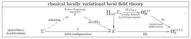
In summary, from the perspective of the topos over partial differential equations, the traditional structure of local Lagrangian variational field theory is entirely captured by the following diagram:

 

So far, all this assumes that there is a globally defined Lagrangian form $L$ in the first place, which is not in fact the case for all field theories of interest. Notably, it is not, in general, the case for field theories of higher WZW type. However, as the above diagram makes manifest, for the purpose of identifying the classical equations of motion, it is only the variational Euler differential $\mathrm{EL} := \delta_V L$ that matters. But if that is so, the variation being a local operation, then we should still call equations of motion $\mathcal{E}$ locally variational if there is a cover $\{U_i \to E\}$ and Lagrangians on each patch of the cover $L : U_i \to \mathbf{\Omega}^p+1_H$, such that there is a globally defined Euler-Lagrange form $\mathrm{EL}$ which restricts on each patch $U_i$ to the variational Euler-derivative of $L_i$

All of the classical field theory still goes through for this case of locally variational field theories [Anderson-Duchamp 80, Ferraris-Palese-Winterroth 11].

But when going beyond classical field theory, the Euler-Lagrange equations of motion $\mathcal{E}$ are not the end of the story. As one passes to the quantization of a classical field theory, there are further global structures on $E$ and on $\mathcal{E}$ that are relevant. These are the action functional and the Kostant-Souriau prequantization of the covariant phase space. For these one needs to promote a patchwise system of local Lagrangians to a horizontal $p$-gerbe connection. This we turn to in the next article.

Click For Forum Comments