Physical Applications of the “Tan Rule”

Introduction

Every secondary school student who has encountered trigonometry in his/her Math syllabus will most likely have come across the sine, cosine, and area rules which are typically used to solve triangles in which certain information is supplied and the remainder are to be calculated. Somewhat surprisingly (because it is relatively simple to derive), the “tan rule” is generally not included as part of this particular set of trig tools. Yet, as we hope to demonstrate in this article, this rule can be extremely useful in certain circumstances. Specifically in the instance where two sides and an included angle of a triangle are given.  In this situation, it is impossible to immediately apply the sine rule to determine the remaining angles since neither of the given sides is opposite the given angle. The cosine rule must first be applied to determine the third side and thereafter the sine rule for either (or both) of the remaining angles. However, the tan rule enables us to determine either of the two missing angles without recourse to either the sine rule or the cosine rule.

Derivation of the “Tan Rule”

The following derivation follows in the footsteps of that presented in Appendix A. The latter is a translation (from Stephen Hawking’s book: On the Shoulders of Giants)  of an extract from “Liber Primus” of “De Revolutionibus Orbium Coelestium” written by one Nicolaus Copernicus and published after his death in 1543. It should be appreciated that the ‘theorem’ is older yet since Copernicus derived his geometry from Greek sources notably Euclid and Ptolemy. He (Copernicus) notes however the subsequent introduction of Arabic numerals: “This notation surpasses any other – Greek or Latin – in a certain singular ease of employment and readily accommodates itself to every class of computation.”

In the diagram of triangle ABC below, sides AB (ie c)  and BC (ie a) are given as is the included angle ABC $(\hat{B})$. From point A drop a perpendicular to point D on side BC extended if necessary depending upon whether D falls inside $\;(\hat{C}$ acute) or outside the triangle $\;(\hat{C}$ obtuse). The triangle is now divided into two right triangles ABD and ADC. Since the angle at D is a right angle and $\hat{B}$ is given, we may calculate AD as $c\sin\hat{B}$ and BD as $c\cos\hat{B}$. CD may then be determined as the difference between BC and BD: $a-c\cos\hat{B}$.

(Note that this difference will be negative in the case of $\hat{C}$ being obtuse in which case $\tan\hat{C}$ will be negative as expected).

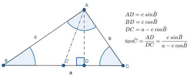Therefore in right triangle ADC, sides AD and CD are given whereby we may determine AC  and angle ACD.

(By Pythagoras’ theorem and the ratio $\tan\hat{C}=\frac{c\sin\hat{B}}{a-c\cos\hat{B}}$ respectively).

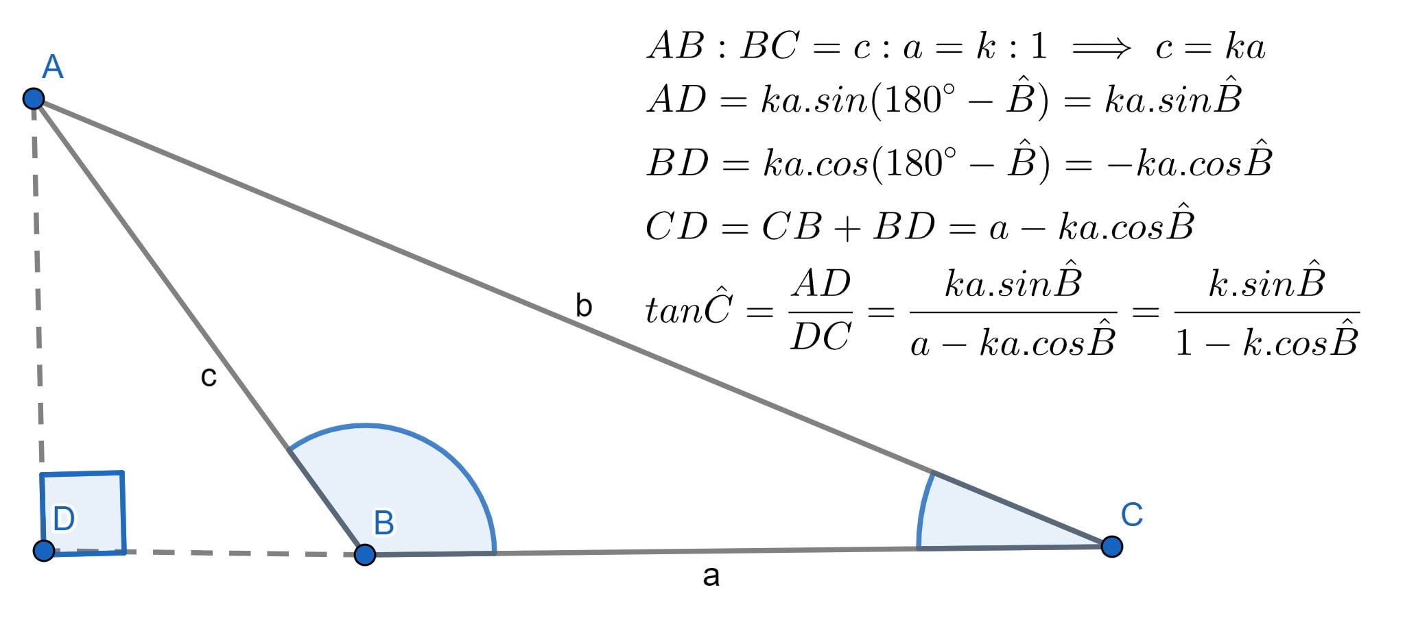
And it will not turn out differently if angle B is obtuse as in the diagram above. The perpendicular dropped from point A to line BC extended creates right triangle ABD in which AD=c sin(180-$\hat{B}$)=c sin$\hat{B}$ and BD=c cos(180-$\hat{B}$)=-c cos$\hat{B}$.

Since BA and BC have a given ratio to each other (BA:BC = c:a = k:1), therefore AB is given (c=ka) in the same parts wherein BD ($=-ka\cos\hat{B}$) and the whole CBD ($=a-ka\cos\hat{B}$) are given.

Accordingly in the right triangle ADC, since the two sides, AD and CD are given, AC (ie b) the side sought and angle $\hat{C}$ are also given.

(by Pythagoras’  Theorem and the ratio: $$\tan\hat{C}=\frac{c\sin\hat{B}}{a-c\cos\hat{B}}=\frac{ka\sin\hat{B}}{a-ka\cos\hat{B}}=\frac{k\sin\hat{B}}{1-k\cos\hat{B}}$$ respectively as before).

An important point to note in the second half ($\hat{B}$ obtuse) of the above derivation is that Copernicus switches from referring to defined sides to a defined ratio of sides. In solving for angle C using the “tan rule”, absolute values of the given pair of sides are not needed as long as one knows the ratio between them. This reflects in the final formula for $\tan\hat{C}$ above and is illustrated in worked examples 1 and 4.

Cyclic Permutation

PF user kuruman notes that once the formula for (say) $\tan\hat{A}=\frac{a\sin{\hat{B}}}{c-a\cos{\hat{B}}}$ is given, the remaining two tan ratios can be found by cyclic permutation, $A\rightarrow B \rightarrow C \rightarrow A$  of the lower and upper case letters. Or if we start from $\tan\hat{A}=\frac{a\sin{\hat{C}}}{b-a\cos{\hat{C}}}$ by similar cyclic permutation in the opposite direction $A\rightarrow C \rightarrow B \rightarrow A$.

Physical Applications

We will examine three physical applications in which the “tan rule” may be usefully employed. The first is in Compton scattering in which a photon is incident upon a stationary electron and there is a transfer of momentum resulting in the photon being ‘scattered’ at an angle dependent on the change in frequency (energy) of the incident and scattered photon. Typically there are two angles to be determined namely that of the scattered photon and that of the electron. Both are measured from the original direction of motion of the incident photon.

The second is in the determination of the angle(s) of projection of a missile if it is to hit a target for which horizontal and vertical coordinates (measured from the point of projection) are known. In this application we will be employing a vector equation $\vec{a}\times\vec{s}=\vec{v}\times\vec{u}$ described in a previous article entitled “Quaternions in Projectile Motion”.

The third is in 2-dimensional elastic collisions between two masses – one moving and one stationary. As in Compton scattering, we find that the post-collision trajectory angles (relative to the pre-collision direction of the moving mass) of the two masses are dependent upon the energy transferred from one to the other as well as (specific to this instance) the ratio of masses. And having determined one angle from an energy relationship, we can determine the other using the tan rule.

It will be seen that there are some interesting similarities between these apparently different physical applications. Momentum and/or impulse are the physical vector quantities in each situation and the angle of deflection is related to energy change. In each case, the 3 vector quantities involved form a triangle in which 2 sides and an included angle are known or can be calculated. A second angle can then be determined by application of the “tan rule”.

Whilst in this article we focus our attention on applications involving momentum and energy,  the “tan rule” is of course as versatile in use as its ‘siblings’ the sine rule and the cosine rule. In the first of the ‘worked examples’ presented, the “tan rule” is illustrated in a problem involving 3 forces in equilibrium. Clearly, the vector sum of such forces will be zero and the associated vector diagram is a closed triangle in which the ratio of two sides along with the included angle are given and we are required to determine a pair of unknown angles. The other 3 worked examples relate to the physical applications mentioned above.

Compton Scattering

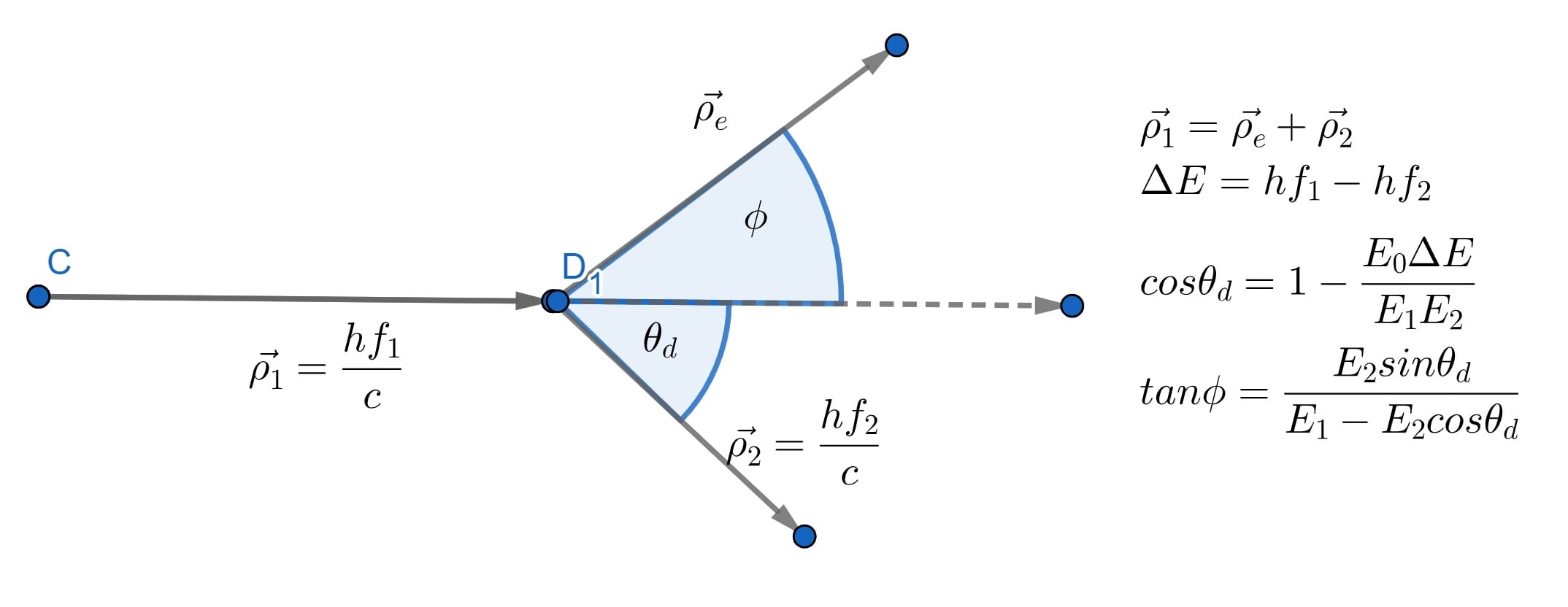
A vector diagram reflecting Compton scattering is shown below. The momentum of the incident photon is equal to the sum of momenta of the scattered photon and impacted electron. It is assumed that the electron is initially at rest.

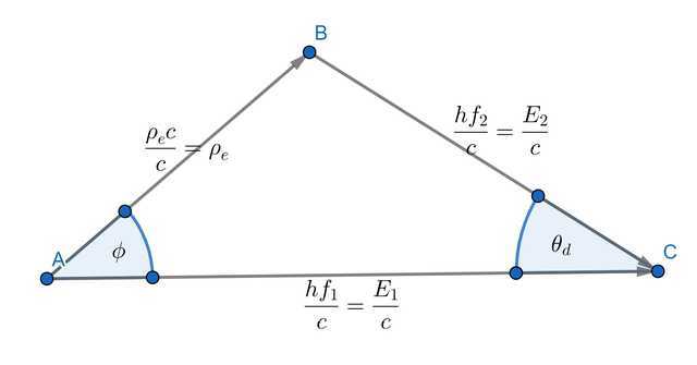
To apply the tan rule to determine the trajectory angle $\phi$ of the electron, we first need the angle of deflection $\theta_d$ between the incident and scattered photon. We could just use a known result, but for completeness, we will include a short derivation thereof.

Final energy of electron: $$E_{ef}=\sqrt{{E_0}^2+(\rho_e c)^2}=E_0+\Delta E$$ where $\Delta E=hf_1-hf_2=E_1-E_2$ ie the difference in energy between incident and scattered photon. $E_0$ is the rest energy of the electron and $\rho_e$ is its momentum. Hence: $$(\rho_e c)^2=(\Delta E)^2+2E_0\Delta E={E_1}^2+{E_2}^2-2E_1E_2+2E_0\Delta E.$$ In the vector diagram above, we multiply all the momentum quantities by constant c to obtain energies and then apply the cos rule to obtain an expression for $\cos\theta_d$: $$ \cos\theta_d=\frac{{E_1}^2+{E_2}^2-(\rho_e c)^2}{2E_1E_2}$$ Substituting for $(\rho_e c)^2$, we obtain: $$\cos\theta_d=\frac{2E_1E_2-2E_0\Delta E}{2E_1E_2}=1-\frac{E_0\Delta E}{E_1E_2}.$$ Since in the above vector diagram all 3 sides of the triangle are known, we could in principle again apply the cos rule to determine angle $\phi$ but it is much simpler to deploy the “tan rule” derived above: $$\tan\phi=\frac{E_2\sin\theta_d}{E_1-E_2\cos\theta_d}.$$

Determination of Projection Angle(s)

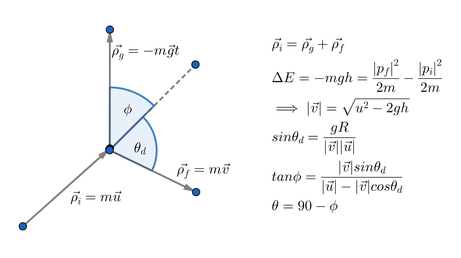
As mentioned above we will be employing the vector equation $\vec{a}\times\vec{s}=\vec{v}\times\vec{u}$ to determine the two possible launch angles for a missile aimed at a target of know co-ordinates (as measured from the launch point). $\vec a$ is acceleration, $\vec{s}$ displacement from launch point  and $\vec u$ and $\vec v$ the initial and final velocities respectively of the projectile. In the case of projectile motion $\vec a=0\;\hat{\textbf{i}} -g\;\hat{\textbf{j}}$ and $\vec s=R\;\hat{\textbf{i}} + h\;\hat{\textbf{j}}$, where R is the horizontal range of the target and h its vertical height above the launch point. Hence  $\vec{a}\times\vec{s}=gR \;\hat{\textbf{z}}$. We can write $\vec{v}\times\vec{u}$ as $|v| |u| \sin\theta_d\; \hat{\textbf{z}}$ where $\theta_d$ is the angle between initial and final velocity vectors. From this we obtain the equation: $$\sin\theta_d=\frac{gR}{|v| |u|}.$$ Here we are following the method described by J. Gibson Winans in an article entitled “Convenient Equations for Projectile Motion” from the American Journal of  Physics. In that article, a construction technique was used to determine launch angles whereas here we adopt an analytic approach employing the “tan rule” described above. Also in that article, the vector equation referred to above arose from the mathematics of quaternion products whereas here we present a derivation based on Newton’s second law applied to angular momentum.

We begin by ‘converting’ the vector equation to an angular momentum equation by the simple expedient of multiplying both sides by the mass m of the projectile: $$m\vec{a}\times\vec{s}=m\vec{v}\times\vec{u}.$$ Then , in the context of projectile motion,  $m\vec{a}\times\vec{s}$ represents the gravitational torque of the projectile relative to its launch point.  Taking our cue from PF User @TSny (who originally identified the physical meaning of the vector equation as described here), we can show that the right hand side of the equation $(m\vec v \times \vec u)$ represents rate of change of angular momentum in accordance with Newton’s second law applied to angular motion: $$L=m\vec{v}\times\vec{s}=m\vec{v}\times\frac{(\vec{v}+\vec{u})t}{2}=\frac{(m\vec{v}\times\vec{u})t}{2}$$

$$\implies \dot L=m\left(\frac{\vec{v}\times\vec{u}}{2}+\frac{(\vec{a}\times\vec{u})t}{2}\right).$$ Writing $\vec a$ as $\frac{\vec v – \vec u}{t}$, the above simplifies to $$\dot L =m\left(\frac{\vec{v}\times\vec{u}}{2}+\frac{\vec{v}\times\vec{u}}{2}\right)=m\vec v \times \vec u$$

Using the “tan rule”, we can now ‘solve’ the following velocity vector diagram to obtain an expression for launch angle(s) in terms of the projectile’s initial velocity, horizontal range to the target, and height of the target. The vector diagram shown is adapted from that which the author first came across in Figure 1 of  PF User kuruman’s Insights article: “How to Master Projectile Motion Without Quadratics.”

$$|v| = \sqrt{|u|^2-2gh}$$

$$\sin\theta_d=\frac{gR}{|u||v|}.$$Noting that the angle of projection $\theta$ is complementary to angle B, we can use the “tan rule” to determine $\tan{\hat B}$ and the reciprocal of this will be equal to $\tan\theta$. $$\tan{\hat B}=\frac{|v|\sin\theta_d}{|u|-|v|\cos\theta_d}\implies \tan\theta=\frac{|u|-|v|\cos\theta_d}{|v|\sin\theta_d}.$$ There will be two solutions (first and second quadrant) for $\theta_d$ and hence two solutions for $\tan\theta$ where $\theta$ is the required launch angle.

2 Dimensional Collisions

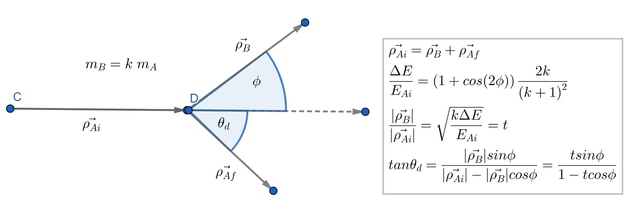
We consider a collision of a moving mass $m_a$ with a stationary mass $m_b$ in which the mass ratio $m_b:m_a=k:1$. If k>1 the collision reflects a lighter mass impacting a heavier and vice versa. The vector diagram (with some modifications to the labelling) is identical to that used for Compton scattering and obeys a similar vector relationship:$$\vec{\rho_{Ai}}=\vec{\rho_{B}}+\vec{\rho_{Af}}$$.  After impact, mass B moves in a direction at an angle $\phi$ to the original direction of mass A. The latter is deflected by an angle $\theta_d$ also measured relative to its original direction.

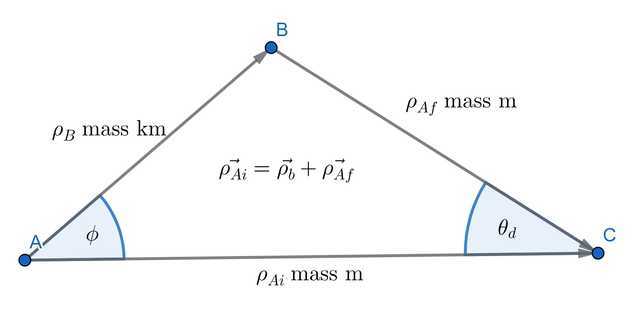
Using a formula obtained in a previous article, we can write an expression for angle $\phi$ in terms of energy and mass ratios. Note that in the following $\Delta E$ refers to the change in energy of moving mass A. Since we are dealing with an elastic collision, all this energy is transferred to mass B. Hence $E_B=\Delta E$. $$1+\cos{2\phi}=\frac{\Delta E}{E_{Ai}}\times\frac{(k+1)^2}{2k}\Longleftrightarrow \frac{\Delta E}{E_{Ai}}=(1+\cos{2\phi}) \times \frac{2k}{(k+1)^2}.$$ We can also write an expression for the momentum ratio $\frac{\rho_{B}}{\rho_{Ai}}$ which will be needed for the calculation of angle $\theta_d$: $$\frac{\Delta E}{E_{Ai}}=\frac{E_B}{E_{Ai}}=\frac{{(\rho_B)}^2/(2km)}{{(\rho_{Ai})}^2/(2m)}\implies\frac{\rho_B}{\rho_{Ai}}=\sqrt{\frac{k \Delta E}{E_{Ai}}}=t.$$ Having obtained angle $\phi$, we can apply the ubiquitous “tan rule” to determine the angle of deflection for mass A: $$\tan(\theta_d)=\frac{\rho_{B} \sin\phi}{\rho_{Ai}-\rho_{B} \cos\phi}=\frac{t\sin\phi}{1-t\cos\phi}$$

Worked Examples

Problem 1

To put the “tan rule” through its paces, we will begin by  “reverse engineering” a typical problem relating to forces in equilibrium whereby an object is suspended from cords attached to the ceiling and we are asked to determine the tension in these chords. The   “Hyperphysics” website supplies us with a “calculator” for such problems:

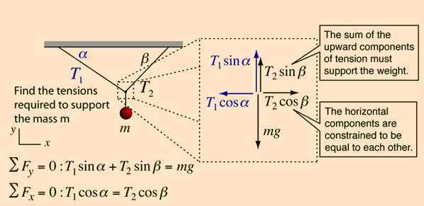
The input data (for the calculator) is the mass of an object and the two angles formed between the chords and the ceiling to which they are fixed. Thus for example if we enter a mass of 10kg and chord angles $\alpha=10.89^{\circ}$ and $\beta=49.11^{\circ}$  measured from the ceiling, the online calculator determines the respective tensions as $T_1=74.076\;N$ and $T_2=111.123\;N$.

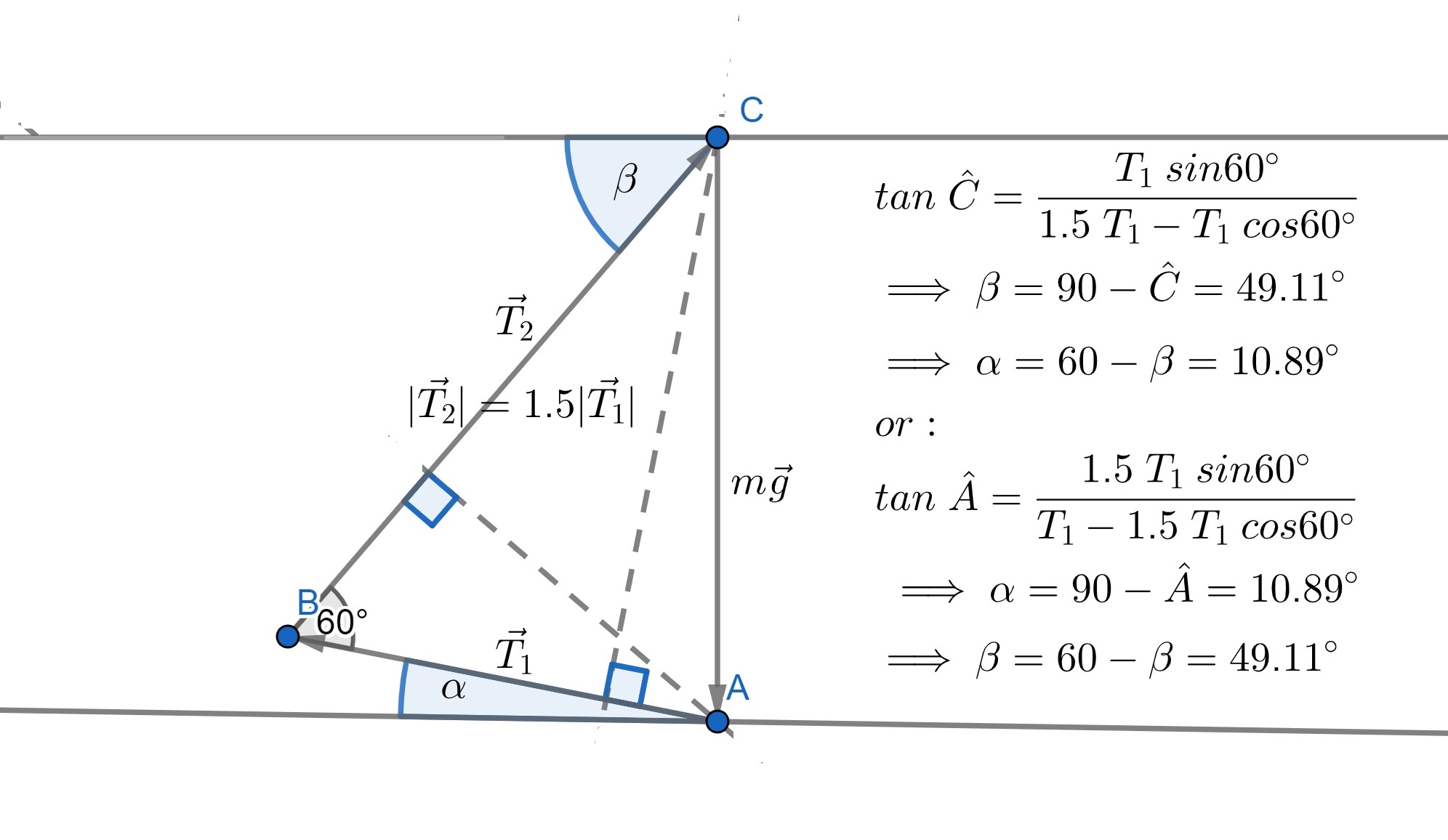
“Reverse engineering” this output we might pose the question: determine the values of angles $\alpha$ and $\beta$ if they sum to $60^{\circ}$ and the ratio of magnitudes $T_2:T_1=1.5$ ? The relevant vector diagram representing $\vec{T_1}+\vec{T_2}+m\vec{g}=0$ is shown below. We include on the diagram calculations (employing the tan rule) to determine angles $\alpha$ and $\beta$. Note that in the formulas for $\tan\hat{C}$ and $\tan\hat{A}$, the variable $T_1$ (reflecting absolute value of tension in the first chord) cancels out. Values of the two tensions are not needed – only the ratio between them.

Problem 2

An 800 keV photon scatters off an initially stationary electron and is subsequently found to have an energy of 650 keV. With reference to the diagram below, determine the photon scattering angle $\theta$  as well as the recoil angle $\phi$ of the electron.

Solution:

$$\Delta E=800\;keV-650\;keV=150 \;keV$$ $$\cos\theta=1-\frac{E_0 \Delta E}{E_1 E_2}=1-\frac{511\;keV\times150\;keV}{800\;keV\times650\;keV}\implies \theta=31.50^{\circ}$$

$$\tan\phi=\frac{E_2 \sin\theta}{E_1 – E_2 \cos \theta} =\frac{650 \sin31.50^{\circ}\;keV}{800\;keV-650\cos31.50^{\circ}\;keV} \implies \phi=54.11^{\circ}$$

Problem 3

A mini projectile launcher in a Physics experiment has a muzzle velocity of 10m/s. With reference to the diagram (and equations) below, determine the two possible projection angles at which the muzzle should be set to hit a target with vector location $(4\;\hat{\textbf{i}}+3\;\hat{\textbf{z}})\;m$ from the launch point.

 

Solution:

$$|\vec{v}|=\sqrt{10^2-2\times9.8\times3}=6.419\;ms^{-1}$$ $$\sin\theta_d=\frac{9.8\;ms^{-2}\times4\;m}{10\;ms^{-1}\times6.419\;ms^{-1}}\implies \theta_d=37.639^{\circ}$$ $$\tan\phi=\frac{6.419\times\sin37.639^{\circ}\;ms^{-1}}{10\;ms^{-1}-6.419\times\cos37.639^{\circ}\;ms^{-1}}=0.797 \implies \phi=38.561^{\circ}\implies\theta=51.439^{\circ}$$ or $$\theta_d=142.261^{\circ}\implies \tan\phi=\frac{6.419\times\sin 142.261^{\circ}\;ms^{-1}}{10\;ms^{-1}-6.419\times\cos142.261^{\circ}\;ms^{-1}}=0.260$$ $$\implies \phi=14.568^{\circ} \implies \theta=75.432^{\circ}$$

Plots of the projectile trajectories for both of these angles are shown below. As can be seen, both are right on target!

Problem 4

Mass A (m kg) impacts stationary mass B (2m kg). After the collision, the trajectory of mass B is at an angle of $45^{\circ}$ to the original direction of mass A.  With reference to the diagram and equations below, determine the angle of deflection of mass A resulting from the collision.

Solution

We are given mass ratio k=2 and $\phi=45^{\circ}$ and can therefore determine the energy ratio $\frac{\Delta E}{E_{Ai}}$ and from that the momentum ratio. Apply the tan rule thereafter to determine the required angle of deflection. $$\frac{\Delta E}{E_{Ai}}=(1+\cos90^{\circ})\frac{2(2)}{(1+2)^2}=\frac{4}{9}$$ $$t=\sqrt{2\times\frac{4}{9}}=\frac{2\sqrt{2}}{3}$$ $$\tan\theta_d=\frac{2\sqrt2\sin45^{\circ}}{3-2\sqrt2\cos45^{\circ}}=2 \implies \theta_d=63.43^{\circ}$$

Summary and Conclusion

In this article, we have introduced the “tan rule” and have employed it to solve problems in areas as apparently diverse as Compton scattering, projectile motion and 2-dimensional elastic collisions. The particular approach used to solve launch angle problems in projectile motion has some interesting similarities with that used to determine deflection angles in Compton scattering and elastic collisions. The base vector quantities in all cases are momentum/impulse. In all three cases, there is an exchange of momentum (and consequently energy) which is related to the post-collision angle of deviation.

In the case of Compton scattering, the momentum “impulse” arises from a collision between the photon and a stationary electron (imparting momentum to the latter) whereas in the case of projectiles there is a gravitational “impulse” mgt, albeit spread over a distinct time interval. However, the “impulse” parameter was not specifically required for the determination of deflection angles (photon and electron in Compton scattering) or launch angle(s) (in projectile motion). Employing energy considerations and the “tan rule” in both cases circumvented the need to determine impulse.

Acknowledgements

I would like to thank PF users vanhees71 , berkeman and Charles Link for taking the time to read through this article and either provide a brief comment or a “like” – both are greatly appreciated! I hope that as a result of such scrutiny, this article will be ‘up to standard’ for publication. It goes without saying that without  Greg there would be no Physics Forums and probably no place to publish the various articles I have been able to write and publish here. I greatly appreciate the encouragement and support he always provides.

In relation to the projectile motion application mentioned in this article, my exploration of the intriguing vector equation $\vec{a}\times\vec{s}=\vec{v}\times\vec{u}$ would never have begun without having come across PF user kuruman’s article “How to Master Projectile Motion without Quadratics.” PF user kuruman did not stop at bringing this equation to our attention but also asked some probing questions about its physical meaning which I later relayed to the forums here. I should also add that PF user kuruman kindly agreed to do a “pre-check” of this article as a result of which the derivation of the  “tan rule” is presented with all the rigour of its distinguished source (as best I can interpret it anyway!).  At his suggestion, I  included an additional worked example by way of forces in equilibrium to further illustrate the versatility of the “tan rule”.

PF User TSny provided an excellent answer to the query concerning the physical meaning (of the vector product equation) and I need to make it clear that the above derivation showing $\dot{L}=m\vec v \times \vec u$ is his particular insight. It is perhaps worth noting that the mathematics of the relationship $\vec{a}\times\vec{s}=\vec{v}\times\vec{u}$ preceded its physical interpretation. For that, we should perhaps also thank none other than William Rowan Hamilton, the “founding father” of quaternions.

As with the previous article on “Quaternions in Projectile Motion”, I would like to thank the American Association of Physics Teachers for kindly granting me permission to make use of material from the American Journal of Physics article on “Convenient Equations for Projectile Motion” by J.Gibson Winans. (see References section below).

Last but by no means least we should mention a certain Nicolaus Copernicus thanks to whom we today have an earth rotating about the sun whereas previously the reverse was the world’s considered wisdom!

References

[1]	Nicolaus Copernicus. De Revolutionibus Orbium Coelestium. 1543. [http | bib ]
[2]	S. Hawking. On The Shoulders Of Giants. Running Press, 2003. [ bib | http ]
[3]	J.Gibson Winans. Convenient Equations for Projectile Motion: American Journal of Physics: Vol 29, no 9.https://aapt.scitation.org/doi/abs/10.1119/1.1937861?journalCode=ajp, February 1961. (Accessed on 08/21/2021). [ bib ]
[4]	PF User Kuruman. How to Master Projectile Motion without Quadratics.https://www.physicsforums.com/insights/how-to-master-projectile-motion-without-quadratics/, November 2020. (Accessed on 06/17/2021). [ bib ]
[5]	HyperPhysics. Force equilibrium. http://hyperphysics.phy-astr.gsu.edu/hbase/fcab.html. (Accessed on 08/21/2021). [ bib ]

 

Appendix A

But now let the given angle ABC be acute, and also let it be comprehended by the given sides AB and BC.

And from point A drop a perpendicular to BC extended if necessary, according to whether it falls inside or outside the triangle, and let it be AD. By this perpendicular the two right triangles ABD and ADC are distinguished, and since the angles in ABD are given – for D is a right angle, and B is known; therefore AD and BD are given by the table as subtending angles A and B whereof AB, the diameter of the circle has diameter 200000 parts. And in the same ratio wherein AB was given in length, AD and BD are given similarly; and CD which is the difference between BC and BD, is given also.

Therefore in the right triangle ADC, the sides AD and CD being given, AC the side sought, and angle ACD is given according to what has been shown above.

Liber Primus Page 39

And it will not turn out differently if angle B is obtuse. For the perpendicular AD dropped from point A to straight-line BC extended makes the triangle ABD have its angles given. For angle ABD, which is exterior to angle ABC, is given and $\hat{D}=90^{\circ}.$ Therefore sides BD and AD are given in the parts whereof AB has (length) 200000. And since BA and BC have a given ratio to one another, therefore AB too is given in the same parts wherein BD and the whole CBD are given.

Accordingly in the right triangle ADC, since the two sides AD and CD are given, side AC and angle ACB which were sought for, are also given.

Appendix B

The following link leads to an extract (0 to 12 degrees) from the “table” referred to in Appendix A above.  Introducing the table Copernicus wrote: “Nonetheless I think it will be enough if in the table we give only the halves of chords subtending twice the arc, whereby we may concisely comprehend in the quadrant what it used to be necessary to spread out over the semicircle.”

In effect, this is a table of sine values referenced to a ‘unit circle’ having a radius of 100000 units. The reader may verify the accuracy thereof by evaluating 100000 sin(x) on a calculator and comparing the result to the corresponding table entry. For example against 7 degrees, we find an entry 12187 as compared to  $100000\;\sin(7^{\circ})=12186.9$.

Liber Primus Page 30