How to Solve Projectile Motion Problems in One or Two Lines

Introduction

We show how one can solve most, if not all, introductory-level projectile motion problems in one or maybe two lines. To this end, we forgo convention.  We demote clock time $t$ to a parameter of secondary importance and ditch the independence of motion in the vertical and horizontal directions.

Starting from first principles, we develop two primary equations that relate five “basic” parameters to each other: $\Delta x$, $\Delta y$, $v_{0x}$, $v_{0y}$ and $v_y$ (standard definitions).  We view the solution of projectile motion problems as equivalent to solving a system of five equations with the five basic parameters as the five unknowns.  Once the system is solved, the time of flight, if one must have it, is just the ratio $\Delta x/v_{0x}$.

To sharpen the implementation of the primary equations, we recombine them to derive three auxiliary shortcut equations that facilitate the identification of equation parameters with given variables.  Finally, we derive a sixth equation to be used with parameter optimization in projectile motion that bypasses differential calculus.  Problems drawn from the PF archives illustrate how to apply the equations.

Equation framework

The two primary equations

We start with the standard transformation for the acceleration in an arbitrary direction $s$, $$a_s=\frac{dv}{dt}=\frac{dv}{ds}\frac{ds}{dt}=v_s\frac{dv_s}{ds}\implies v_s dv_s=a_s ds $$  When the acceleration is constant and non-zero,$$\int_{v_{0s}}^{v_s}v_s dv_s=a_s\int_{s_0}^s ds \implies v_s^2-v_{0s}^2=2a_s(s-s_0)=2a_s\Delta s.$$When the acceleration is zero in the $s$-direction, $v_s=\text{constant}.$

Now in 2d motion the position coordinates $x$ and $y$ vary simultaneously.  Specifically for projectile motion, when we set $s=y$ and $a_y=\text{-}g$, we obtain the familiar equation $$\begin {align}\Delta y=\frac{v_{0y}^2-v_y^2}{2g}.\end {align}$$However, when we set $s=x$, all we get is $v_x=\text{const.} = v_{0x}$ which is not very informative until we realize that the independence of the vertical and horizontal motion occurs as a result of using time $t$ as parameter. The parametric expressions $x(t)$ and $y(t)$ automatically synchronize the horizontal and vertical projections of the projectile’s position: at any single value of time $t$, evaluation of these expressions gives the projections along each axis.

Synchronization is not automatic, however, when one writes expressions for the variation of the coordinates as functions of velocity.  To achieve synchronization in this case, we first note that, in time interval $\Delta t$, the projectile’s displacement is simultaneously $\Delta x$ along the horizontal and $\Delta y$ along the vertical axis.  Using the definition of the average velocity in a given direction, we then write $$\Delta t=\frac{\Delta x}{\bar v_x}= \frac{\Delta y}{\bar v_y}.$$ With $\bar v_x=v_{0x}$ and $\bar v_y=\frac{1}{2}(v_{0y}+v_y)$, we get the “synchronization” equation $$\begin{align}\frac{\Delta x}{v_{0x}}=\frac{2\Delta y}{v_{0y}+v_y}.\end{align} $$This equation contains all five basic parameters and combines the horizontal and vertical directions.

The three auxiliary equations

To obtain the first auxiliary equation we substitute $\Delta y$ from equation (1) into (2). After some obvious algebra, $$\begin{align}\Delta x=\frac{v_{0x}(v_{0y}-v_y)}{g}=\frac{|\vec v \times \vec v_0|}{g}. \end{align}$$We have encountered this equation in a previous insight.

To obtain the second auxiliary equation we solve equation (2) for $v_y$ and substitute the result in (3), $$g\Delta x=v_{0x}(v_{0y}-v_y)= v_{0x}\left(2v_{0y}-2v_{0x}\frac{\Delta y}{\Delta x}\right).$$Defining angle $\theta$ as the projection angle and $\varphi$ as the angle formed between the instantaneous position vector and the $x$-axis, we have $v_{0y}=v_{0x}\tan\!\theta$ and $\dfrac{\Delta y}{\Delta x}=\tan\!\varphi$ in which case the equation above can be rewritten as, $$\begin{align}\frac{\Delta x}{\tan\!\theta-\tan\!\varphi}=\frac{2v_{0x}^2}{g}.\end{align}$$The astute reader will recognize this as a rearrangement of the equation for the parabola $y(x),~$obtained by eliminating parameter $t$ from the SUVAT 2d equations.  Here, we have replaced $y$ by $\Delta y=\Delta x \tan\!\varphi$ and $x$ by $\Delta x$.

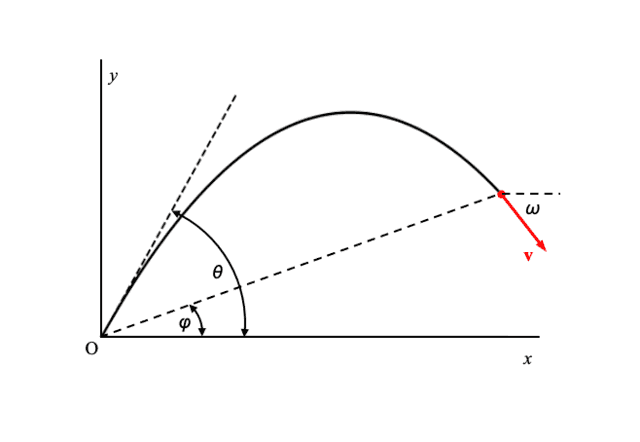
We now obtain the third and final auxiliary equation.  We introduce angle $\omega$ formed between the velocity vector and the horizontal axis. From equation (2), $$\frac{\Delta y}{\Delta x}=\frac{1}{2}\left(\frac{v_{0y}}{v_{0x}}+\frac{v_{y}}{v_{0x}}\right).$$With $\dfrac{v_{y}}{v_{0x}}=\tan\omega$ and the previous definitions for the other two slopes, $$\begin{align}\tan\!\varphi=\frac{1}{2}(\tan\!\theta+\tan\!\omega).\end{align}$$The figure below illustrates the angles in equation (5).  Note that tangents of angles below the horizontal must be the negatives of themselves in this equation.

Examination of the two primary equations shows that five parameters determine uniquely the parabolic path: the two instantaneous displacements, $\Delta x$ and $\Delta y$, the two components of the initial velocity, $v_{0x}$ and $v_{0y}$ (or the initial speed $v_0$ and the angle of projection $\theta$) and the vertical component of the instantaneous velocity $v_y$.

Thus, the solution to any projectile problem requires the determination of these five “basic” parameters. It is formally equivalent to solving a system of five equations and five unknowns.  The primary equations are two of the five.  Although the auxiliary equations can be used, they do not count because they are derived from the primary two. Thus, the task is to establish three additional equations.  These would be relations between the five basic parameters and physical quantities provided in the statement of the problem.

Projection angle optimization

Projectile motion problems sometimes require finding the optimum projection angle at which the horizontal range or the vertical distance or the initial speed are at an extremum.   Here we derive an optimization relation that applies to all such problems.

Using a couple of trigonometric identities, we group and rewrite the trigonometric functions in equation (4) as $$2\cos^2\!\theta(\tan\!\theta-\tan\!\varphi)=\frac{2\cos\!\theta\sin(\theta-\varphi)}{\cos\!\varphi}=\frac{\sin(2\theta-\varphi)-\sin\!\varphi}{\cos\!\varphi}. $$Equation (4)  becomes $$\sin(2\theta-\varphi)=\dfrac{g \Delta x \cos\!\varphi}{v_0^2}+\sin\!\varphi=c ~~~\left(c\equiv \dfrac{g \Delta x \cos\!\varphi}{v_0^2}+\sin\!\varphi\right).$$

There are two projection angles at which the right-hand side has the same value because the equation $\sin(2\theta-\varphi)=c$ has two solutions:

$2\theta-\varphi=\arcsin(c)\implies \theta_1=\frac{1}{2}(\arcsin(c)+\varphi)$
$2\theta-\varphi=\pi-\arcsin(c)\implies \theta_2=\frac{1}{2}(\pi-\arcsin(c)+\varphi)$

Thus, $\theta_1+\theta_2=\dfrac{\pi}{2}+\varphi.$  The implicit basic variables on the right hand side of the definition for $c$ are $\Delta x$, $\Delta y$ and $\sqrt{v_{0x}^2+v_{0y}^2}.$  Choosing one of these to optimize involves fixing the other two and finding the projection angle $\theta_{\text{extr.}}$ at which the chosen variable is at an extremum. It, being a function of $\theta$, is double-valued when there there are two different projection angles resulting in the same $c$. It will be single-valued, when the two projection angles are no longer different: $\theta_1=\theta_2=\theta_{\text{extr.}}$  It follows that, $$2\theta_{\text{extr.}}=\frac{\pi}{2}+\varphi\implies \theta_{\text{extr.}}=\frac{\pi}{4}+\frac{\varphi}{2}~;~\tan\!\theta_{\text{extr.}}=\dfrac{1}{\cos\!\varphi}+\tan\!\varphi=\sqrt{1+\tan^2\!\varphi}+\tan\!\varphi.$$

With $\tan\!\theta = \tan\!\theta_{\text{extr.}}$ and $\tan\!\varphi=\dfrac{\Delta y}{\Delta x}$ in equation (4), we obtain the optimization condition $$\begin{align}\sqrt{(\Delta x)^2+(\Delta y)^2 }+\Delta y=\frac{v_0^2}{g}.\end{align}$$ Examples 3, 4 and 5 below illustrate its implementation in problem-solving.

We now investigate what happens when we substitute $\tan\!\theta_{\text{extr.}}$ in equation (5).  $$2\tan\!\varphi = (\frac{1}{\cos\!\varphi}+\tan\!\varphi)+\tan\!\omega\implies \tan\!\omega=\frac{\sin\!\varphi-1}{\cos\!\varphi}. $$ Then, $\tan\!\theta_{\text{extr.}}\times\tan\!\omega=\dfrac{1+\sin\varphi}{\cos\!\varphi}\times\dfrac{\sin\!\varphi -1}{\cos\!\varphi}=\dfrac{\sin^2\!\varphi-1}{\cos^2\!\varphi}=-1.$

Hence, at optimization, the initial and final velocity vectors are perpendicular to each other irrespective of the optimized variable.

Examples

We have selected problems from the PF archives that do not explicitly ask for the time of flight. We have also filtered out problems that involve the use of equation (3) because these were examined in an earlier insight.  When one has solved for the displacements and velocities, one can always find the time of flight by evaluating either side of equation (2).

1. Basketball
(Inspired by this original post.)

A basketball player is standing on the floor at a distance $R$ from the basket. At what initial speed angled at $\theta$ with the horizontal must he throw the ball so that it goes through the hoop without striking the backboard? The basket height is at height $d$ above the floor and the ball leaves the player’s hand at height $h$ above the floor ($d > h$).

Use equation (4) with $\tan\!\varphi=\dfrac{d-h}{R}$ : $$\frac{R}{(\tan\!\theta-\frac{d-h}{R})}=\frac{2v_{0}^2\cos^2\!\theta}{g}\implies~v_0=\frac{R}{\cos\!\theta}\sqrt{\frac{g}{2[R\tan\!\theta-(d-h)]}} .$$

2. Archery
(Inspired by this original post.)
You are watching an archery tournament when you start wondering how fast an arrow is shot from the bow. Remembering your physics, you ask one of the archers to shoot an arrow parallel to the ground. You find the arrow stuck in the ground distance $L$ away, making angle $\omega$ with the ground.

(a) Find the initial speed of the arrow $v_0$.

Use equation (4) with $\tan\!\theta=0~\implies~ v_{0x}=v_0.$  $$\frac{L}{(0-\tan\!\varphi)}=\frac{2v_{0}^2}{g}\implies v_0^2=\frac{gL}{-2 \tan \!\varphi}.$$ From equation (5), $\tan\!\varphi=\frac{1}{2}\tan\!\omega.$  This gives $v_0=\sqrt{\dfrac{gL}{- \tan\!\omega}}.$

Note: The radical appears to be imaginary but it is not.  Angle $\omega$ is below the horizontal, hence the numerical value for $\omega$ substituted in the equation must be negative which makes the radical real.

(b) Find the initial vertical distance $y_0$ from the arrow to the ground.

Substitute directly in equation (1):   $\Delta y=\dfrac{0^2-v_y^2}{2g}=\dfrac{-v_0^2\tan^2\!\omega}{2g}.$

$y_0=|\Delta y|=\dfrac{v_0^2\tan^2\!\omega}{2g}.$

3. Incline landing
(Inspired by this original post.)
You fire a ball with an initial speed $v_0$ at an angle $\theta$ above the horizontal on an incline, which is itself inclined at an angle $\varphi$ above the horizontal  ($\theta > \varphi$).  Ignore air resistance.
(a) Find the distance $d$ measured along the incline, from the launch point to the point where the ball strikes the incline.

Use equation (4) directly with $\Delta x=d~\cos\!\varphi$ : $$\frac{d~\cos\!\varphi}{(\tan\!\theta-\tan\!\varphi)} =\frac{2v_{0}^2\cos^2\!\theta}{g}\implies~d=\frac{2v_0^2\cos^2\!\theta}{g\cos\!\varphi}(\tan\!\theta-\tan\!\varphi) .$$

(b) What angle $\theta$ gives the maximum range, measured along the incline? What is the maximum value?

We know already that the optimized projection angle is $\theta_{\text{extr.}}=\dfrac{\pi}{4}+\dfrac{\varphi}{2}.$   To find the maximum distance up the incline, in the optimization condition (6) we let $d_{\text{max}}=\sqrt{(\Delta x)^2+(\Delta y)^2 }$ and set $\Delta y =d_{\text{max}}\sin\!\varphi.$  Then  $$d_{\text{max}}+d_{\text{max}}\sin\!\varphi=\frac{v_0^2}{g} \implies d_{\text{max}}=\frac{v_0^2}{g(1+\sin\!\varphi)}.$$

4. Pitched roof
(Inspired by this original post.)
What is the minimum velocity required to throw a ball over a house with a pitched roof given dimensions a, b and c as shown in the figure?

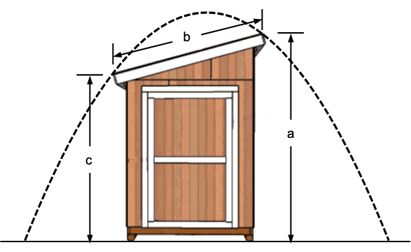
We consider the motion from one corner of the roof at height $c$ where the speed is $v_c$ to the other corner at height $a$.  We note that $\sqrt{(\Delta x)^2+(\Delta y)^2 }=b$ and $\Delta y=a-c$.  The optimization condition (6) becomes $$b+(a-c)=\frac{v_c^2}{g}\implies v_c^2=g(a+b-c)$$ To find $v_0$, we write equation (1) from the starting point on the ground to the corner at height $c$, $2gc=v_{0y}^2-v_{cy}^2$ and then add and subtract $v_{0x}^2$ on the right hand side to get $2gc=v_0^2-v_c^2 \implies v_0^2=v_c^2+2gc=g(a+b+c)$.

5. Up the wall
(Inspired by this original post.)
A projectile, launched at A with initial velocity $v_ 0$ at angle $\theta$, impacts the vertical wall at B.  Compute the angle $\theta$ that will maximize the height $h$ of the impact point. What is this maximum height?

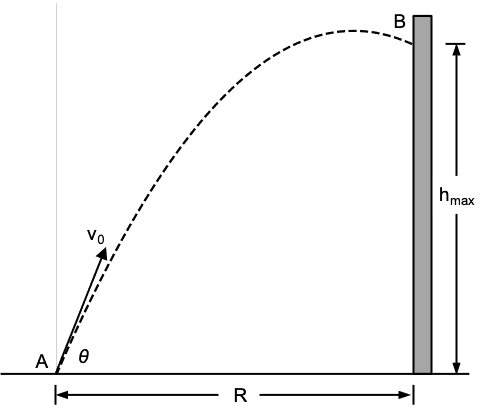In the optimization condition (6), we substitute $\Delta y=\Delta x \tan\!\varphi$ and divide both sides by $\Delta x$, $$\sqrt{1+\tan^2\!\varphi }+\tan\!\varphi=\frac{v_0^2}{g\Delta x}.$$We have already seen in the angle optimization section that $\tan\theta_{\text{extr.}} =\sqrt{1+\tan^2\!\varphi}+\tan\!\varphi.$  Thus, with $\Delta x=R$, the projection angle that will maximize the height is given by $\tan\theta_{\text{extr.}}=\dfrac{v_0^2}{gR}.$

To find the value of the maximum height, we let $\Delta y=h_{\text{max}}$ and set $\Delta x=R$ in the optimization condition.  Then $$\sqrt{h_{\text{max}}^2+R^2}+h_{\text{max}}=\frac{v_0^2}{g} \implies h_{\text{max}}=\frac{v_0^4-g^2R^2}{2gv_0^2}.$$

6. Increasing distance
(Inspired by  this original post.)
A projectile is thrown from a point on the ground at an angle $\theta$ above the horizontal. It moves in such a way that its distance from P is always increasing from its launch until it falls back to the ground. Find all the possible values of $\theta$ with which the projectile could have been thrown. You can ignore air resistance.

Clearly, the magnitude $|\Delta \vec r|$ will keep increasing as long as the angle between the displacement and velocity vectors is less than $90^o$, which implies the dot product condition $$v_{0x}~\Delta x+v_y~\Delta y  > 0.$$Using equation (5), we rewrite $v_y=v_{0x}\tan\omega=v_{0x}(2\tan\!\varphi-\tan\!\theta)$ in which case the dot product condition becomes $$\Delta x+~(2\tan\!\varphi-\tan\!\theta)\Delta y  > 0 \implies 1+\tan\!\varphi(2\tan\!\varphi-\tan\!\theta)>0.$$To find at what angle $\varphi$ the left side crosses zero, we solve the quadratic in $\tan\!\varphi$ to get$$\tan\!\varphi=\frac{1}{4}\left(\tan\!\theta\pm\sqrt{\tan^2\!\theta-8}\right).$$To answer the question posed by the problem, we note the following:

1. When motion starts, distance $d$ from the origin is increasing.  Any decrease must occur when the dot product goes through zero and becomes negative, i.e. the angle between the position and the velocity vector becomes greater than $90^o.$  This can only happen after the projectile has reached maximum height.
2. When $\tan\!\theta < 2\sqrt{2}$, there is no value of $\theta$ for which the dot product is negative. Thus, for $\theta < \arctan(2\sqrt{2}) = 70.5^o$, the magnitude of the displacement vector will increase during the entire flight.
3. When $\tan\!\theta > 2\sqrt{2}$ the magnitude of the displacement vector decreases for values of $\tan\!\varphi$ between the two roots of the quadratic.

Discussion

The equations we provided here contain no new physics but bring to the table an alternate point of view, a plan B that makes problem-solving more direct than the conventional plan A.   Plan B eliminates the preliminary step of finding the time of flight, it facilitates the assessment and identification of what is given, what is asked for, and how to get to the answer, it shortens the algebraic steps with equations that combine horizontal and vertical variables and it affords parameter optimization without the need for a function to optimize with respect to the projection angle using calculus.

Equation (4) is particularly useful because it incorporates most of the key substitutions and stands out as the workhorse equation.  It brings together the initial and final parameters of the motion and transforms, as we have seen, most problems into one-liners.

The reader might wish to compare the parabolic equation of plan A with its alter ego in plan B, equation (4): $$y(x)=y_0+x~\tan\!\theta-\frac{g x^2}{2 v_0^2\cos^2\!\theta}~;~~\frac{\Delta x}{\tan\!\theta-\tan\!\varphi}=\frac{2v_{0x}^2}{g}.$$The equations are different in appearance, yet the only mathematically noteworthy difference between them is that $y_0=0$ in the equation on the right.

Nevertheless, appearances can give rise to bias. The equation on the left has the gravitas of a parametric equation in which $x$ and $y$ are the independent and dependent variables.  As such, it invites doing the necessary algebra and substitutions on the right-hand side leaving the left-hand side untouched. This is especially true in cases requiring variable optimization where the urge to set $\dfrac{dy}{d\theta}=0$ and proceed from there is irresistible.

In contrast, neither side of the equation on the right has a single isolated variable.  The variables are treated on an equal footing.  This makes their identification with physical parameters in the problem easier to establish and invites algebraic manipulations and substitutions on both sides. As we have seen, the simple argument that we used to obtain the optimization condition is easier to deduce with the equation on the right than the one on the left. Perceptions matter.

Finally, the importance of angle $\varphi$ cannot be overstated.  We have seen through the examples how central it is in solving projectile motion problems quickly and efficiently.  Yet, this angle is largely ignored and noticed only when it is misidentified as the projection angle $\theta$.

Summary

The formulation of projectile motion in two dimensions is easy to summarize in terms of two one-dimensional motions occurring simultaneously in two independent directions (plan A), however, its use often leads to circuitous problem-solving and unnecessary steps.  We have presented an alternate formulation of projectile motion that considers the independence of the motion components and the time of flight of secondary importance.     We have seen that restructuring the formulation of the starting equations (plan B) leads to a significant reduction of the algebra and a simplification of how one perceives the problem and establishes the correspondence between motion variables and given quantities.

Acknowledgment

I am grateful to @neilparker62 for keeping me honest during the assembly of this insight.  This article would not have been written without @neilparker62. His goading and prodding encouraged me to dig deeper, beyond his and my earlier insights on projectile motion.  He also brought to my attention the J. Gibson Winans article after I mentioned to him the optimization condition.  Thank you @neilparker62!

Endnote

Some of the equations presented here have been derived before, albeit in a different form, using quaternions in the article “Convenient Equations for Projectile Motion” by J. Gibson Winans [American Journal of Physics 29, 623 (1961); doi: 10.1119/1.1937861].  Most of this insight was completed before the Gibson article came to the author’s attention.