How to Master Projectile Motion Without Quadratics

Introduction

In a homework thread a while back a PF member expressed dismay along the lines of “Oh no, not another boring projectile motion problem.” Admittedly, I shared the member’s sentiments at the time.  Yet after some thought, I concluded that it is the unvarying recommended strategy of the genre that makes it boring: (a) Write down the  SUVAT equations ada[ted for projectile motion; (b) find the time of flight from the vertical motion equation; (c) use the time of flight to find whatever else you need. “Perhaps,” I thought, “relief from ennui might be found if one forsakes the traditional approach altogether.  How about a formulation of projectile motion based on geometry and trigonometry that allows analysis without quadratic equations?” This tutorial is a streamlined account of how to do it.

The velocity triangle

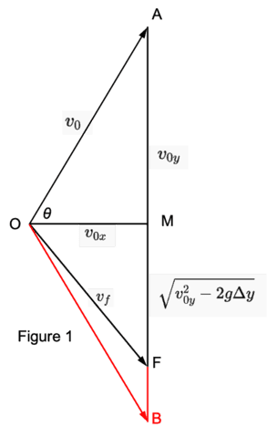
In 2-d projectile motion without air resistance, the equation relating the velocity $\vec v_{\!f}$ at time $t_{\!f}$ and the initial velocity $\vec v_0$  is $$\vec v_{\!f}=\vec v_0+\vec g~t_{\!f}.$$The three vectors participating in the equation form a closed triangle the sides of which are $OA = v_0$, $OF = v_{\!f}$ and a third vertical side $AF = g~ t_{\!f}$ (see figure 1).  Triangle OAF in the figure corresponds to a projectile that is at positive vertical displacement $\Delta y$ at time $t_{\!f}$ after reaching maximum height. I call this the velocity triangle; its geometric construction from three given lengths is outlined in Appendix I. Triangle OAB is another velocity triangle corresponding to the projectile returning to launch level and is drawn for later reference.

The time of flight

An arrow from the origin O to any point on the vertical line segment $AF$ represents the instantaneous velocity vector.  As time increases, its tip moves at a constant rate $g$ from point A to F. When it is at point M, the projectile is at maximum height. The speed of the projectile is the same at pairs of points symmetrically disposed about M. The two times at which the speed of the projectile is the same are given by $t_{\!f} =\frac{AM\pm MF}{g}$. Segment $AM=v_{0y}=\sqrt{2gh_{max}}$ where $h_{max}$ is the maximum height to which the projectile rises.  To obtain segment $MF$ we note that, after an object is released from rest and drops by height $H’$, its speed is $\sqrt{2g H’}$. Here we have $H’ = h_{max} – \Delta y$, so that $MF =\sqrt{2g (h_{max}-\Delta y)}=\sqrt{v_{0y}^2-2g \Delta y}$.  Thus, the two times at which the projectile is at displacement $\Delta y$ and has equal speeds are given by $$\begin{align}t=\frac{v_{0y}\pm \sqrt{v_{0y}^2-2 g\Delta y}}{g}.\end{align}$$

When the projectile drops below the launch point, the vertical displacement $\Delta y$ (a signed quantity) is negative therefore $(-2g\Delta y)$ in the equation must be replaced with $(2g |\Delta y|)$.

From the two right triangles OMA and OMF we also have $$\begin{align}& v_0^2=v_{0x}^2+v_{0y}^2 ~\Rightarrow~v_0=\sqrt{v_{0x}^2+v_{0y}^2} \nonumber \\ & v_{\!f}^2=v_{0x}^2+v_{\!fy}^2= v_{0x}^2+v_{0y}^2-2g\Delta y~\Rightarrow~v_{\!f}=\sqrt{v_0^2-2g \Delta y}. \nonumber \end{align} $$ This last result, also obtainable from work-energy considerations, shows that $v_{\!f}$ depends only on the initial speed $v_0$ and the vertical displacement $\Delta y.$

The range

We define the range $R$ as the horizontal distance from the origin when the projectile is at vertical displacement $\Delta y.$ Mathematically, $R = v_{0x} t_{\!f}.$ Using the velocity triangle, $$\begin{align}R=v_{0x}\times\frac{AM+MF}{g}=\frac{v_{0x}}{g}\left[v_{0y}+\sqrt{v_{0y}^2-2 g\Delta y}\right]=\frac{v_{0x}v_{0y}}{g} \left[1+\sqrt{1-\frac{2g \Delta y}{v_{0y}^2}}\right].\end{align}$$In the special case where the projectile returns to launch level ($\Delta y =0$), the expression reduces to the familiar result, $$\begin{align}R_0=\frac{2v_{0x} v_{0y}}{g}.\end{align}$$

The product $(v_{0x})(AF)$ is twice the area $A$ of the velocity triangle which can also be written as the cross product, $2A = |\vec v_0 \times \vec v_{\!f}|.$ Thus, the range can be written compactly as $$\begin{align}R=\frac{|\vec v_0 \times \vec v_{\!f}|}{g}.\end{align}$$For fixed displacement $\Delta y$ and varying projection angle $\theta$, this is maximum when $\vec v_0$ is perpendicular to $\vec v_f.$  Then the expression for the maximum range is$$\begin{align}R_{\text{max}}=\frac{v_0 v_{\!f}}{g}=\frac{v_0\sqrt{v_0^2-2 g\Delta y}}{g}.\end{align}$$To find the angle of projection $\theta_{\text{max}}$ at which the range is maximum, we observe that, in this case, the velocity triangle is a right triangle and angle AOM (or $\theta_{\text{max}}$) is equal to angle OFA. Thus,$$\tan(\theta_{\text{max}})=\frac{OA}{OF}= \frac{v_0} {v_{\!f}} =\frac{v_0}{\sqrt{v_0^2-2g \Delta y}}.$$

The “other” range and “other” projection angle

With parameter $u=\tan\theta$, the quadratic equation relating the range and the tangent of the projection angle can be written as$$\begin{align}\frac{g^2}{v_0^2} (u^2+1)R^2-2 g  u R + 2 g\Delta y  =0.\end{align}$$It is a quadratic in either $u$ or $R$ and can be used to find either (1) the ranges of the two trajectories that pass through height $\Delta y$ at fixed projection angle or (2) the two angles of projection that put the projectile at $\Delta y$ when launched from fixed horizontal distance $R$. We will proceed to find these quantities without solving this equation.

1. To find the “other” range, consider the trajectory when the projectile goes past height $\Delta y$ and lands at the launch level at the other side of $\Delta y$. The resulting velocity triangle is AFB in Figure 1. The “other” range is the additional horizontal distance covered by the projectile. It is represented in Figure 1 as twice the area of triangle OFB and obtained algebraically by subtracting equation (2) from equation (3).  Combining this difference and equation (3) in one equation gives the two reduced ranges at fixed angle $\arctan(u)$:$$R=\frac{v_0^2}{g}\frac{u}{(u^2+1)}\left[1\pm \sqrt{1-\frac{(u^2+1)}{u^2}\frac{2g \Delta y }{ v_0^2}}\right].$$As expected these are the two solutions of quadratic equation (6).

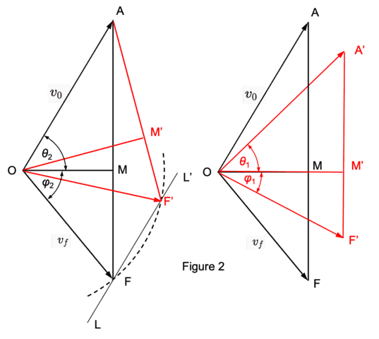
2. We will first find the “other” angle geometrically by constructing the “other” triangle. We are seeking a triangle that has sides $v_0$ and $v_{\!f}$ and area equal to the area of triangle OAF. To construct this triangle (see Figure 2 left),
At point F draw line LL’ parallel to $v_0.$  Draw a circle (dashed arc in Figure 2, left) of radius $v_{\!f}$ centered at point O. Label as F’ the other point where the circle intersects line LL’.

We note that

1. Triangle OAF’ (Figure 2, left) is the desired other triangle: it has sides $v_0$ and $v_{\!f}$ by construction while twice its area is the perpendicular distance between parallel lines $v_0$ and LL’ multiplied by $v_0$, same as for triangle OAF.
2. Angle OAF is opposite to $OF$ in triangle OAF and is also complementary to given projection angle $\theta_2.$ Likewise, angle OAF’ is opposite to $OF’$ in triangle OAF’ and is complementary to the “other” projection angle. Thus, the desired “other” projection angle $\theta_1$ is formed between segment $OA$ and $OM’$, the perpendicular from point O to $AF’.$

To be properly displayed, triangle OAF’ is rotated about point O to bring side $AF’$ along the vertical (triangle OA’F’ in Figure 2, right). The computation of the “other” angles $\theta_1$ and $\varphi_1$ from $\theta_2$ and $\varphi_2$ using the two equal-area triangles in Figure 2, right is relegated to Appendix II.

The position triangle

If we draw the median from point O to the opposite side AF in Figure 1, the original velocity triangle is divided in two halves (Figure 3, left). Looking at the top half, OAC, we see that $AC = \frac{1}{2}gt_{\!f}$. We redraw this top triangle (Figure 3, right) imagining that it has been rescaled by an overall factor $t_{\!f}$. Then $OA = v_0 t_{\!f}$ and $AC = \frac{1}{2}g{t_{\!f}}^2$. The third side, $OC$, is identified as the final position of the projectile considering that in Figure 3, right we have the vector diagram of $\vec r_{\!f}=\vec v_0 t_{\!f}+\frac{1}{2}\vec g{t_{\!f}}^2.$

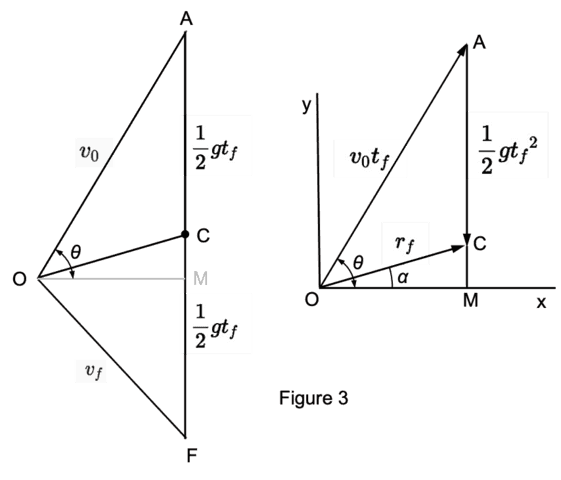
Length $CM$ is the displacement $\Delta y$. Constructing the position triangle from the velocity triangle is analogous to finding the displacement by integrating the velocity.

Beyond being a curiosity, the position triangle can serve as a useful tool for solving problems that cannot be addressed by a velocity triangle construction. Consider the problem in which a projectile is fired up a plane inclined at angle $\alpha$ relative to the horizontal. The projection angle is $\beta$ relative to the incline and we are seeking the landing distance $d$ up the incline. The traditional strategy is to find the trajectory parabola by eliminating $t_{\!f}$ from the horizontal and vertical position equations, find the horizontal distance $x_{\!f}$ at which the parabola intersects the straight line $y = x \tan\alpha$, find the final height $y_{\!f}$ and finally use the Pythagorean theorem to find the required distance $d$. This two-page solution can be reduced to two lines using the position triangle.

Solution
We are looking for the length of $r_{\!f}$ in Figure 3 right. We apply the law of sines to the position triangle OAC. For the three angles involved, we have $\sin(COA) = \sin\beta$, $\sin(OAC) = \cos\theta = \cos(\alpha + \beta)$ and $\sin(ACO) = \sin(\frac{\pi}{2}+\alpha) = \cos\alpha$. The law of sines provides two independent equations. The first equation gives the time of flight,$$\frac{g t_{\!f}^2}{2 \sin (\beta )}=\frac{v_0 t_{\!f}}{\cos (\alpha )}~\Rightarrow~ t_{\!f}=\frac{2 v_0 \sin (\beta )}{g \cos (\alpha )}.$$The second equation gives the distance up the incline, $$\frac{d}{\cos (\alpha +\beta )}=\frac{v_0 t_{\!f}}{\cos (\alpha )}~\Rightarrow~ d=\frac{2 v_0^2 \sin (\beta ) \cos (\alpha +\beta )}{g \cos ^2(\alpha )}.$$

Afterthoughts

We have seen how it is possible to find what is usually asked in projectile motion problems without recourse to quadratic solutions but by using simple trigonometry and geometry. The velocity triangle formulation may be viewed as a form of linearization that eliminates the need for solving quadratics. Furthermore, we have seen how the position triangle can be used to set up the kinematics equations through the use of the law of sines. The result that the range is proportional to the area of the velocity triangle introduces a great simplification that affords, as we have seen, not only a quick calculation of the range but also range maximization without calculus. This makes the velocity triangle a useful pedagogical tool because it allows students to look “under the hood” and see the time evolution of the velocity vector. Drawing a unique velocity diagram tailors the solution to a specific physical situation and results in a unique answer.  By contrast, the quadratics normally provide two answers one of which must be rejected although “it comes out of the equation.”

Furthermore, the formulation provides a different perspective by putting the final velocity on an equal footing with the initial velocity. It exploits the well-understood but unused (in projectile motion) fact that the final speed is strictly determined by the initial speed and the vertical displacement. Equally unused, untaught, and not even assigned as a “show that” exercise is Equation (4) which identifies the range as the magnitude of the cross product of the initial and final velocity divided by $g$. It appears that this beautiful equation has been ignored because of adherence to the quadratic formulation as the only method for addressing problems in projectile motion.

Authoring this article liberated me from this bias and rounded my understanding of projectile motion by connecting dots that needed connecting. I no longer find projectile motion boring.

Appendices

I. Construction of velocity triangle OAF.

We assume that the input parameters, namely the initial velocity components and a measure of the vertical displacement, are given straight-line segments.

1. Pick one of the given line segments and label it $OM$ ($=v_{0x}$).  Pick the longer of the remaining two segments and label it $AM$ ($=v_{0y}$). Label the last segment $\sqrt{2g \Delta y}.$
2. Draw right triangle OMA with right sides $v_{0x}$ and $v_{0y}$ as seen in Figure 1.
3. Draw a separate right triangle (not shown in Figure 1) with one right side $\sqrt{2g \Delta y}$ and hypotenuse $v_{0y}.$ Label the other right side $MF$.  Note that $MF =\sqrt{v_{0y}^2-2g \Delta y}.$
4. Add vertical segment $MF$ to form vertical side $AF.$

II. Computation of “other” angles $\theta_1$ and $\varphi_1.$

The projection angle $\theta_2$ and landing angle $\varphi_2$ shown in triangle OAF are, in terms of the given quantities, $${\theta_2}=\cos^{-1} \left[\frac{v_{0x}}{\sqrt{v_{0x}^2+v_{0y}^2}}\right];~~\varphi _2=\cos^{-1}\left[\frac{v_{0x}}{\sqrt{v_{0x}^2+v_{0y}^2-2g \Delta y }}\right].$$The equality of the ranges implies the equality of the areas of triangles OAF and OA’F’. If we express the areas as cross products and set them equal we obtain, after cancellations$$\sin(\theta_1+\varphi_1)=\sin(\theta_2+\varphi_2).$$For $\theta_2 \neq \theta_1$ and $\varphi_2\neq \varphi_1$ this implies $\theta_1+\varphi_1 = \dfrac{\pi}{2} – (\theta_2+\varphi_2)$ in which case $$\cos(\theta_1+\varphi_1)= – \cos(\theta_2+\varphi_2).$$

Refer to Figure 2 right and apply the law of cosines to each triangle.

$(A’F’)^2=v_0^2 – 2 v_0 v_{\!f}\cos(\theta_1+\varphi_1)+v_{\!f}^2;~~(AF)^2=v_0^2 – 2 v_0 v_{\!f} \cos(\theta_2+\varphi_2)+v_{\!f}^2.$

From the relation between the cosines of the sums of the angles, it follows that $(A’F’)^2=(AF)^2+4\cos(\theta_2+\varphi_2).$  With $OM = v_0 \cos\theta_2$ and $OM’ = v_0 \cos\theta_1$, the equality of the triangles’ areas is expressed as$$A’F’ v_0\cos\theta_1=AF v_0\cos\theta_2~\Rightarrow~\cos\theta_1=\frac{AF\cos\theta_2}{\sqrt{(AF)^2+4v_0v_{\!f}\cos(\theta_2+\varphi_2)}}.$$The “other” angle $\varphi_2$ is given by $$\cos\varphi_1=\frac{v_0\cos\theta_1}{v_{\!f}}=\frac{v_0 AF\cos\theta_2}{v_{\!f}\sqrt{(AF)^2+4v_0 v_{\!f}\cos(\theta_2+\varphi_2)}}.$$