A Poor Man’s CMB Primer: Cosmic Acoustics

 

Before decoupling, photons and charged particles were in good thermal contact: though the primordial plasma might have varied in temperature from place to place, the photons and baryons were in local thermal equilibrium and shared a common temperature. If some physical process caused the baryons to heat up in some place, this temperature change was communicated swiftly to the photons in that place, and vice versa. And so when the universe cooled through recombination and the photons broke free from the charged plasma, they carried away with them a record of the plasma temperature at each point in the universe. We observe this temperature record today on Earth as the cosmic microwave background: a two-dimensional shell called the last scattering surface. It is the spherical cross-sectional map of the 3-dimensional plasma sea at the time of decoupling¹ with a radius, $d_{\rm ls}$, determined by the distance that light has traveled since decoupling, which is very nearly equal to the size of today’s observable universe. The CMB record is therefore a projection of sorts, like a shadow, of actual physics going on in the 3-dimensional universe. In this post, we’ll learn what the 2-dimensional pattern of temperature anisotropies on the last scattering surface tells us about the nature of the baryon-photon plasma at the time of decoupling.

To get started, let’s consider a simplified universe of two dimensions. Suppose the baryon-photon plasma is spread out across a sheet of paper, and let’s set up plane waves of wavelength $\lambda$ in the plasma: these will be compressional waves, and the higher-density, compressed regions will heat up relative to lower-density, rarefied regions. The photons are liberated at decoupling and flow across the cosmos. Those that arrive at Earth today originated a distance $d_{\rm ls}$ from Earth—in this 2-dimensional flatland, this is the radius of the last scattering circle. To our flatlander, the last scattering circle appears as in Figure 1 with alternating hot and cold spots,

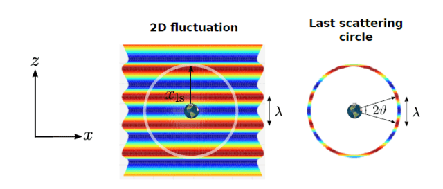
Fig 1. Left: a 2-dimensional example of a single temperature fluctuation of wavelength $\lambda$. Right: to a resident of a flat Earth, the fluctuation results in a 1-dimensional last scattering circle; the fluctuation subtends an angle $\vartheta$.

Notice that the angular separation of the pair of hot spots in Figure 1 very nearly determines $\lambda$ in a flat universe (a fine assumption for now) through the simple relation $d_{\rm ls} \approx \lambda/2\vartheta$, illustrating a key theme: spatial inhomogeneity becomes angular anisotropy! As you can see from Figure 1, though, the angular separation of adjacent hot and cold spots varies as you go around the circle and so this simple relation isn’t suitable for understanding generally how the wavelength of a plasma wave can be recovered from the angular anisotropy it imparts on the last scattering circle.

Of course, the same thing happens with a 3-dimensional wave. To correctly relate a 3-dimensional fluctuation to its 2-dimensional spherical imprint, we need to consult an important result, probably most pertinent to scattering problems, that allows us to write a plane wave as a combination of spherical waves. It’s called a plane wave expansion,
\begin{equation}
\label{pwe}
e^{i{\bf k}\cdot{\bf r}} = 4\pi \sum_{\ell = 0}^\infty \sum_{m=-\ell}^\ell i^\ell j_\ell (kr) Y_{\ell m}(\hat{\bf r}) Y^*_{\ell m}(\hat{\bf k}),
\end{equation}
where $\hat{\bf k}$ is the wave vector, $\hat{\bf r}$ points from Earth to a location on the last scattering sphere, and the $j_\ell$’s are spherical Bessel functions. We see immediately that a single plane wave gives rise to a series of angular fluctuations—not just one—with the spherical Bessel functions controlling how much the plane wave contributes on each angular scale $\vartheta \approx \pi/\ell$.

As an easy example, we’ll consider a 3-dimensional plane wave propagating in the $\hat{\bf z}$-direction with a wavelength $\lambda = 2d_{\rm ls}/3$, as in Figure 1 (where, though Figure 1 was used as a 2-dimensional example, we can view it as the cross-section of a 3-dimensional plane wave in the $xz$-plane.) In this case, $m=0$ and Eq. (\ref{pwe}) simplifies considerably,
\begin{equation}
e^{i{\bf k}\cdot{\bf r}} = 4\pi \sum_{\ell = 0}^\infty \sqrt{\frac{2\ell +1}{4\pi}}j_\ell(kr) Y_{\ell 0}(\hat{\bf r}),
\end{equation}
with only the zonal spherical harmonics appearing in the sum. Working out the first few terms of the series we see that a plane wave with $\lambda = 2d_{\rm ls}/3$ contributes most strongly to anisotropies on the last scattering surface through multipoles $\ell = 7$ and $\ell = 8$,

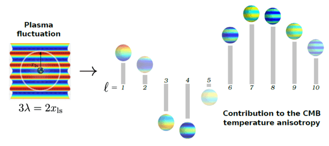
Fig 2. A single plane wave generates anisotropy across a range of angular scales on the last scattering surface. The contribution to each multipole is determined by the pre-factor $\sqrt{\frac{2\ell +1}{4\pi}}j_\ell(kr)$. Contributions to multipoles $\ell > 10$ drop off to zero rapidly.

Furthermore, and conversely, the multipole $\ell = 7$ receives it greatest contribution from the plane wave with $\lambda = 2d_{\rm ls}/3$, where $j_7(kr)$ has its global maximum. The spherical Bessel functions are decaying oscillating functions, with subsequent local maxima corresponding to the diminishing contributions from fluctuations with ever smaller wavelengths,

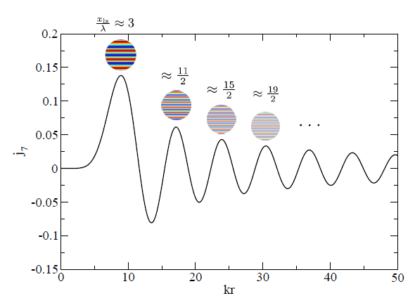
Fig 3.  The spherical Bessel function or order $\ell$ has a global maximum near $kr \approx \ell$, so fluctuations on the scale $k$ contribute most to multipole $\ell$. Fluctuations with larger $k$ make ever-decreasing contributions via the local maxima of the function.

In general, for a fluctuation with wavenumber, $k$, the rule-of-thumb is that it contributes most to the multipole for which $kr \approx \ell$ (and, conversely, that this multipole receives its greatest contribution from this mode)², and therefore, a fluctuation of wavelength $\lambda$ contributes most strongly to anisotropies on the last scattering surface with an angle $2\vartheta \approx \lambda/d_{\rm ls}$. This is the result that we obtained naively for the 2-dimensional fluctuation in Figure 1, though we see now that a single fluctuation manifests as anisotropies at all angular scales, with a magnitude controlled by the $j_\ell$’s. Finally, to round out the discussion, a plane wave with arbitrary wave vector, ${\bf k} = (k_x,k_y,k_z)$, gives rise to non-zonal ($m\neq 0$) anisotropies.

To summarize so far: we have shown that there is a good correspondence between plasma fluctuations on a scale $k$ and temperature anisotropies on an angular scale $\vartheta \approx \pi/\ell \approx \lambda(2d_{\rm ls})^{-1}$, and this is cool because it means we can use the CMB to study the baryon-photon plasma on various scales before decoupling³. As we learned in the last post, the CMB exhibits temperature correlations across a decent sweep of angular scales, and therefore we expect a spectrum of plasma fluctuations to have existed across a corresponding range of wavelengths at decoupling. So, what were these fluctuations?

Let’s go back to the days before recombination, when the universe was ruled by the baryon-photon plasma, well-described as a perfect fluid⁴ of density $\rho$. Imagine perturbing the baryon density slightly in some places. What might happen? We know that an overdensity will tend to gravitationally attract more baryons, and so maybe we expect the overdensity to grow a bit. But as the overdensity grows, the tight coupling between baryons and photons ensures more frequent scattering, which causes the plasma to warm up, which promotes the diffusion of plasma back out of the overdensity. We expect this kind of undulation of the plasma at a basic conceptual level: gravity pulls matter in, and radiation pressure drives it back out. Formally, we can describe it using a set of equations from Newtonian physics,
\begin{eqnarray}
\label{cont}
\dot{\rho} + {\nabla}\cdot(\rho {\bf v}) &=& 0, \\
\label{eul}
\dot{{\bf v}} + ({\bf v}\cdot{\nabla}){\bf v} &=& -\frac{1}{\rho}{\nabla}{\bf p} – {\nabla}\phi, \\
\label{pois}
{\nabla}^2 \phi &=& 4\pi G\rho.
\end{eqnarray}
The first is the well-known continuity equation, which says that the rate of change of density within a closed volume is balanced by the flow rate of material across the volume boundary; ${\bf v}$ is the fluid 3-velocity. The next is Euler’s equation of fluid dynamics, which describes how fluid flow rates and directions are affected by thermodynamic work and external forces, where here the work is due to pressure gradients, ${\nabla}{\bf p}$, and the relevant external force is gravity, represented by the Newtonian potential $\phi$. The last is Poisson’s equation relating the Newtonian gravitational potential to the matter density. Why Newtonian physics when cosmology is under the purview of general relativity? First, we’re going to look at perturbations of the quantities in Eqs. (\ref{cont}-\ref{pois}), and so we’ll be dealing with weak gravitational fields and relatively small energy densities. Second, we’ll initially only be studying perturbations with wavelengths smaller than the cosmological horizon at the time of the last scattering—what this means will be made clear shortly. A third reason is conceptual clarity: bringing the full sophistication of general relativity to bear on such tiny, small-scale fluctuations is inhumane and will distract us from the physics.

As written, Eqs. (\ref{cont}-\ref{pois}) describe Newtonian fluid dynamics in static spacetime. Expansion is made manifest in these equations by the simple fact that it causes the fluid to move, and the farther away it is, the faster it moves. This is Hubble’s law, written ${\bf v} = H{\bf x}$, where $H$ is the Hubble parameter⁵, defined in terms of scale factor as $H=\dot{a}/a$ and ${\bf x}$ is the physical distance between the observer and fluid element. We additionally reconsider our position variable in expanding space: because physical length scales grow along with the expansion, $x \propto a$, we write $x = ar$, where $r$ is the comoving distance. It is simply a yardstick that grows along with the expansion, so that objects whose motion is due solely to the expansion have constant comoving positions, $\dot{r} = 0$. This change to comoving coordinates is largely anticipatory, as we will soon need to keep constant labels on things that are growing with the expansion. We suppose that the fluid velocity is due solely to the expansion (i.e. it is locally at rest), and so we make the substitution ${\bf v} = Ha{\bf r}$ in Eqs. (\ref{cont}-\ref{pois}) to go from static to expanding spacetime. Eqs. (\ref{cont}-\ref{pois}) become
\begin{eqnarray}
\label{cont2}
\dot{\rho} + 3H\rho &=& 0, \\
\label{eul2}
\dot{{\bf v}} + 3H{\bf v} &=& -\frac{1}{a\rho}{\nabla}{\bf p} – \frac{1}{a}{\nabla}\phi, \\
\label{pois2}
{\nabla}^2 \phi &=& 4\pi G a^2\rho,
\end{eqnarray}
where we have used the fact that ${\nabla}_{\rm r}\cdot {\bf r} = 3$, where ${\nabla}_{\rm r} = a {\nabla}$ is the derivative with respect to comoving coordinates. Now, we’re interested in solving Eqs. (\ref{cont2}-\ref{pois2}) for the perturbed quantities, and so we write the fluid density, fluid velocity, and gravitational potential as the sum of a background value and a small perturbation, $\delta x \ll \bar{x}$,
\begin{equation}
\rho({\bf x},t) = \bar{\rho}(t) + \delta \rho({\bf x},t), \,\,\,\,\,\,\,\,\,\, {\bf v}({\bf x},t) = \bar{{\bf v}}(t) + \delta {\bf v}({\bf x},t), \,\,\,\,\,\,\,\,\,\, \phi({\bf x},t) = \bar{\phi}(t) + \delta \phi({\bf x},t).
\end{equation}
Putting these into Eqs. (\ref{cont2}-\ref{pois2}) and keeping only first-order terms (e.g. discarding terms like $\delta \rho \delta {\bf v}$), gives
\begin{eqnarray}
\label{dp}
\dot{\delta} &=& -\frac{1}{a}{\nabla}\cdot \delta {\bf v}, \\
\label{dv}
\dot{\delta {\bf v}} + H\delta {\bf v} &=& -\frac{1}{a\rho_0}{\nabla}\delta {\bf p}- \frac{1}{a}{\nabla}\delta\phi, \\
\label{dphi}
{\nabla}^2 \delta \phi &=& 4\pi Ga^2\bar{\rho}\delta,
\end{eqnarray}
where we’ve introduced the density contrast, $\delta = \delta \rho/\bar{\rho}$. This is the quantity that we’re after, and we can arrive at an equation of motion for $\delta$ by combining Eqs. (\ref{dp}-\ref{dphi}) as follows: take $\frac{{\rm d}}{{\rm d}t}$ of Eq. (\ref{dp}), substitute in the divergence (${\nabla}\cdot$) of Eq. (\ref{dv}), and use Eq. (\ref{dphi}) to eliminate $\delta \phi$, giving
\begin{equation}
\label{perts}
\ddot{\delta} + 2H \dot{\delta} + \left(-\frac{c_s^2}{a^2}{\nabla}^2 – 4\pi G\bar{\rho}\right)\delta = 0,
\end{equation}
where $c_s = \delta p/\delta \rho$ is the speed at which compressional waves travel through the fluid; it’s referred to as the sound speed of the fluid. At fixed time, the quantity $\delta$ describes how the energy density of the cosmological fluid varies from place to place: it charts the hills and valleys of the baryon-photon plasma. By taking the Fourier transform of the density contrast,
\begin{equation}
\label{ft}
\delta ({\bf x},t) = \int \frac{{\rm d}^3 k}{(2\pi)^3}\delta_k(t) e^{-i{\bf k}\cdot{\bf r}},
\end{equation}
we can examine the evolution of the individual, component frequencies of the overall density contrast. This is precisely the philosophy behind the maneuver in the last post, where the spatial temperature anisotropy field was decomposed into its spherical harmonics to study phenomena on individual angular scales. Dropping Eq. (\ref{ft}) into Eq. (\ref{perts}) yields an equation for an individual Fourier “$k$-mode”,
\begin{equation}
\label{kmode}
\ddot{\delta_k} + 2H \dot{\delta_k} + \left(\frac{c_s^2 k^2}{a^2} – 4\pi G\bar{\rho}\right)\delta = 0,
\end{equation}
where $k$ is a comoving wavenumber: it is a static label attached to a Fourier mode with a physical wavelength evolving as $\lambda_{\rm phys} = 2\pi/k_{\rm phys} = 2\pi a/k$. It’s convenient because it allows us to package all the time dependence of $\delta( {\bf x},t)$ into the Fourier amplitudes, $\delta_k(t)$. Equation (\ref{kmode}) is intriguing, if expected: it is the Bessel equation (in some disguise) describing damped oscillations. The damping is simply a result of the expanding space, manifested via the friction term, $2H\dot{\delta_k}$. Let’s ignore the damping for a moment, in which case we have solutions,
\begin{equation}
\delta_k(t) \sim e^{i\omega t}, \,\,\,\, \omega = \sqrt{\frac{c_s^2 k^2}{a^2} – 4\pi G \bar{\rho}}.
\end{equation}
It turns out that the wavelike behavior is not assured, because $\omega$ can be imaginary depending on the tug-of-war between terms under the square root sign. If $c_s^2 k^2/a^2 \gg 4\pi G \bar{\rho}$, then the restoring force of radiation counterbalances the driving force of gravity, and we get oscillations about equilibrium: $\delta_k(t)$ evolves as a damped, nearly plane wave. If, however, the second term dominates, then gravity overwhelms the restoring radiation pressure, and $\delta_k$ grows under gravitational instability. Which force dominates depends on the size of the fluctuation, with the critical scale given by Jeans length,
\begin{equation}
\label{Jeans}
\lambda_J = \sqrt{\frac{\pi c_s^2}{G\bar{\rho}}}.
\end{equation}
Fluctuations larger than this are sufficiently massive for gravity to overcome the radiation pressure and the amplitude grows, otherwise, the fluctuation oscillates as a sound wave. Now, the largest length scale of relevance to sound waves is that of the fundamental tone: to use a musical metaphor, a fundamental tone on a guitar has a wavelength, $\lambda_1$, twice the size of the oscillator—the string. Here, the oscillator is the plasma, and its effective “length” is set by the distance that sound has traveled from the big bang up until the time of decoupling. This is an important distance, known as the sound horizon, $d_s$. Naively, one might expect the proper distance to the horizon to be $c_s t_{dec}$, where $t_{dec}$ is the time after the big bang that decoupling occurs, but this is wrong because it neglects the effect of expansion which aids in moving the wave along, resulting in a larger distance traveled. Consider the comoving velocity of the sound wave, that is, the velocity of the wave as measured by a yardstick increasing in length along with the expansion, $\dot{r} = c_s/a$. The distance traveled in comoving units is then
\begin{equation}
\label{compart}
r = c_s \int_0^{\eta_s} {\rm d}\eta = c_s \int_0^{t_{dec}} \frac{{\rm d}t}{a(t)}.
\end{equation}
In integrating from the Big Bang up until decoupling, the universe passes from being dominated by radiation to being dominated by non-relativistic matter, and the sound speed, $c_s^2 = \partial p/\partial \rho$, is sensitive to this change in the equation of state. Here we will assume that the universe is matter-dominated throughout the domain of the integral in Eq. (\ref{compart}), allowing us to take $c_s$ constant. To proceed we need to understand how $a(t)$ varies with time in a matter-dominated universe; for this, we solve the Friedmann equation,
\begin{equation}
\label{FE}
H^2 = \frac{8\pi G}{3} \rho,
\end{equation}
which relates the expansion rate to the homogeneous and isotropic density, with $\rho \propto a^{-3}$, since matter densities vary inversely with volume, $V \propto a^{3}$. We find that in a matter-dominated universe the scale factor grows as a power-law, $a(t) \propto t^{2/3}$, and with this result we can integrate Eq. (\ref{compart}) to find $r(t_{dec}) = d_s = 3c_s t_{dec}/a_{dec}$. The proper distance, $x = ar$, traveled by a sound wave from the dawn of the universe until decoupling is then $x(t_{dec}) = 3c_s t_{dec}$, shorter than the Jeans length⁶.

Now, if we know the comoving distance to the last scattering surface, $d_{\rm ls}$, we can determine the angular scale corresponding to the fundamental tone, via $\vartheta \approx \pi/\ell \approx \lambda_1(2d_{\rm ls})^{-1} = d_s/d_{\rm ls}$. To find it, we calculate the distance that photons have traveled from decoupling up to the present day; it’s a very similar calculation to that used to find $d_s$, except that photons travel at the speed of light, $c=1$, and the limits of integration change:
\begin{equation}
\label{compart2}
r = \int_{\eta_s}^{\eta_0} {\rm d}\eta = \int_{t_{dec}}^{t_0} \frac{{\rm d}t}{a(t)},
\end{equation}
where we’ll again assume a matter-dominated universe throughout. Ignoring the bottom limit of the integration, we find $d_s/d_{\rm ls} = c_s(t_{dec}/t_0)^{1/3}$, and since the photon temperature $T \propto 1/a$ with $a \propto t^{2/3}$, this becomes
\begin{equation}
\frac{d_s}{d_{\rm ls}} = c_s \sqrt{\frac{T_0}{T_{dec}}} \approx \frac{1}{\sqrt{3000}} \approx \frac{1}{55} \approx 1^\circ,
\end{equation}
where we’ve taken $c_s^{-1} = \sqrt{3}$ and $T_0 \approx 3$ K. This is a remarkable result: the sound horizon at decoupling subtends an angle of only $1^\circ$, a tiny fraction of the full CMB sky, partitioning correlations into those arising from fluctuations that were within the sound horizon at decoupling, so-called sub-horizon modes, and those with wavelengths larger than the horizon at decoupling so-called super-horizon modes. Correlations on sub-horizon scales are perhaps expected, given the symphony of sound waves spreading across space and other causal processes at work within the horizon; however, correlations across super-horizon scales are beguiling, apparently defying causality. Let’s discuss both in more detail.

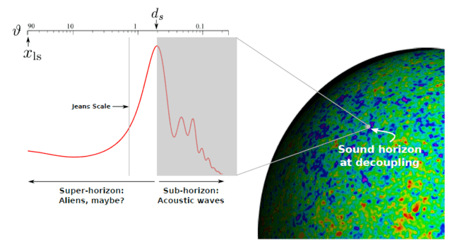
Fig 4. Fluctuations on sub-horizon scales with wavelengths subtending but a tiny $1^\circ$ angle on the surface of the last scattering, oscillated as sound waves until decoupling. Correlations on super-horizon scales reveal the existence of very large-scale fluctuations that are effectively frozen because they’ve evolved only very slowly relative to the age of the universe at decoupling. Those fluctuations in between the Jeans scale and the sound horizon oscillate as acoustic waves but have periods long compared to the age of the universe at decoupling and so haven’t completed even a half cycle by this time.

As Figure 4 illustrates, fluctuations on sub-horizon scales create the signature ripples in the temperature correlation function. The broad central peak at $\ell_1 \approx 180^\circ/1^\circ = 180$ is due to the fundamental tone: sound waves of wavelength $\lambda_1 = 2d_s$ and frequency $f_1 = c_s/\lambda_1 = 2\eta_s$ that have completely compressed once just in time for the “snapshot” at decoupling⁷,

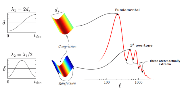
Fig 5. The broad central peak at $\ell_1 \approx 220$ (this differs from $\ell_1 \approx 180^\circ/1^\circ = 180$ above because this spectrum was generated for a more realistic model without the assumption of pure matter domination) due primarily to the fundamental tone with $\lambda_1 = 2d_s$: a sound wave with a wavelength twice the sound horizon at decoupling. The frequency of this wave is $f = 2\eta_s$ and so it has completed just one full compression by decoupling. The $1^{\rm st}$ overtone is also shown, corresponding to a smaller wavelength fluctuation with $\lambda_2 = \lambda_1/2 = d_s$: it has completed one compression and one rarefaction by decoupling, and dominates the strong correlation at $\ell_2 \approx 2\ell_1$. Note that the local minima are not actual extrema, and are instead a result of the fact that the temperature power spectrum is proportional to the squared fluctuation $\Delta T$.

Notice that we don’t use the coordinate time $t$ here to measure the frequency, because the waves are traveling in an expanding space; the quantity $\eta$ is a “time” variable that takes the expansion into account⁸. The peaks on smaller angular scales are due to the higher-frequency overtones: for example, the sound wave with $\lambda_2 = \lambda_1/2$ corresponding to the peak at $\ell_2 \approx 2\ell_1$ has a frequency $f_2 = \eta$ and so will have compressed and rarefied once by decoupling, and the wave with $\lambda_3 = \lambda_1/3$ and frequency $f_3=2\eta/3$ will have compressed, rarefied, and compressed once more by this time. A spectrum of overtones with $\lambda_n = \lambda_1/n$ exists as distinct peaks in the CMB at $\ell_n = n\ell_1$, though at smaller and smaller angular scales these fluctuations get washed out due to various damping phenomena that we’ll discuss later. The idea is that the temperature correlation function peaks on scales where the acoustic waves were at a maximum (compression) or a minimum (rarefaction) at decoupling.

This makes perfect sense if we’re considering the amplitude of only a single wave on each scale, but remember that the correlation on an angular scale, $\ell$, is an ensemble average of many independent fluctuations with different amplitudes (the $a_{\ell m}$’s). One might expect such an unruly collection of oscillations to be most decidedly not correlated. The key is that the fluctuations are independently coherent in phase for each $k$. For example, consider the central peak at $\ell \approx 180$: there are $m = 2\ell + 1 = 361$ independent anisotropies on the last scattering sphere arising from fluctuations that are each just completing one compression at decoupling, i.e. they each look like the top left panel in Figure 5. Why is this? It seems spooky, or at least exceptionally fine-tuned, that each of these independent fluctuations should have coherent phases.⁹

The case is similar for super-horizon fluctuations smaller than the Jeans scale: these are acoustic oscillations that are trying to compress, but simply haven’t had enough time since the Big Bang to complete a half cycle. In keeping with our musical analogy, they are plucked guitar strings that have yet to make a sound. Fluctuations on scales larger still are gravitationally unstable—they are growing, not oscillating—but they have scarcely evolved in the time preceding decoupling and are essentially frozen. These correlations are therefore not a result of any post-big bang casual process: the fluctuations were initialized in a coherent state, seemingly acausally across vast stretches of the cosmos. In the next post, we’ll learn about where these fluctuations came from. It’s a remarkable, near-unbelievable story.

Footnotes

¹By “spherical cross-section” I mean the surface of a ball carved out of a 3-dimensional block of plasma. I like to think of the last scattering sphere as the surface of a scoop taken from a giant tub of delicious ice cream. back
²It is generally stated that this approximation gets better with larger $\ell$. This actually is not true (it gets worse, in the sense that $kr – \ell$ increases with larger $\ell$) and it’s more correct to say that $kr/\ell \rightarrow 1$ as $\ell$ grows. For example, for $\ell < 20$, a given $k$-mode contributes most to multipole $\ell = kr – n$, where $n$ ranges between 2 and 3 for $\ell$ between 2 and 20. We’ll follow convention with this minor caveat in mind. back
³Note that the two $\approx$’s signify different approximations: the first reflects the close but imperfect correspondence between multipole moment $\ell$ and the angular scale, $\vartheta$, of fluctuations it exhibits; the second is the one we just touched on: that the fluctuation of wavenumber $k$ in flat space contributes to angular scales quite near, but not exactly, $\lambda(2d_{\rm ls})^{-1}$. back
⁴A perfect fluid is completely described by its rest mass density and isotropic pressure; it has no viscosity or bad habits and doesn’t conduct heat. back
⁵$H$ gives the logarithmic rate of spatial expansion, but colloquially it’s called simply the expansion rate. back
⁶To see this, take $3H=2/t$ during matter domination and use the Friedmann equation to replace $\bar{\rho}$ in Eq. (\ref{Jeans}) to find $\lambda_1/\lambda_J = 2d_s/\lambda_J \approx 2/3$. back
7 These estimates are based on our assumption of a matter-dominated universe from the Big Bang up until decoupling, and so they don’t match the figures which are hifalutin, actual best-fits to the concordance cosmological model. back
⁸More formally it is called the conformal time, defined ${\rm d}\eta = \int {\rm d}t/a(t)$. It is the time given on a clock that is slowing down with the expansion of the universe. back
9 9 As helpful as the musical analogy has been, the early universe would have made a terrible orchestra. Though the CMB contains a spectrum of nice, phase-coherent harmonic tones, they are spatially incoherent and so would sound like TV static. back