A Poor Man’s CMB Primer: Bumps on a Blackbody

 

Astronomers Arno Penzias and Robert Wilson discovered the cosmic microwave background in 1965. They were not looking for it.

They were using the comically distorted Holmdel Horn Antenna at Bell Labs, New Jersey, to study the reflection of radio waves off NASA balloon satellites. Despite all efforts to remove interference while calibrating the instrument (which included cooling the receiver with liquid helium to a frigid $4\, {\rm K}$, pointing it up and away from the galactic plane to avoid astrophysical contamination, and making frequent trips into the antenna to clean up pigeon poo) a mysterious noise persisted in the data. Penzias and Wilson eventually concluded that the source of the noise was extragalactic, but a shrug of the shoulders was all they could offer in explanation. Its significance soon became clear when the two learned of work by a team of Princeton cosmologists (Dicke, Peebles, Wilkinson, and Roll [1]) who were hunting for the fossilized remains of the universe’s fiery beginnings. The big bang, they reasoned, must have released a tremendous amount of radiation in addition to all the matter making up all the stars and galaxies in the universe. A large amount of expansion since the “primordial fireball” should have cooled this radiation down to only a few dozen Kelvin. Further, they asserted, the spectrum of the background radiation should conform to a near-perfect blackbody, putting it squarely in the microwave band of the electromagnetic spectrum. Squarely, that is, in the laps of Penzias and Wilson.

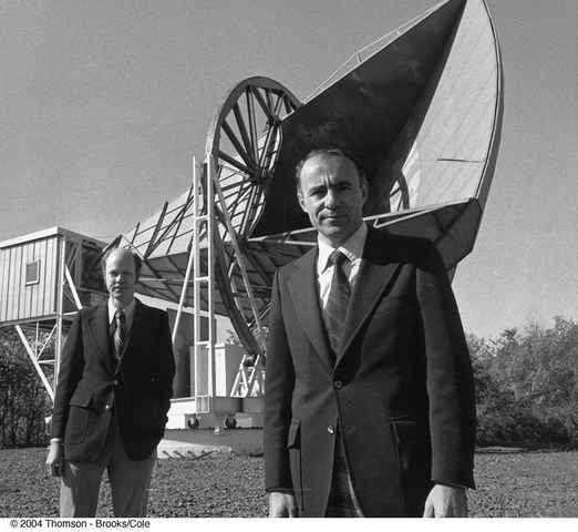
Fig 0. Arno Penzias (front) and Robert Wilson at Holmdel.  Lucky bastards.

It’s worthwhile understanding how the Princeton gang came to expect cold, near-blackbody¹ background radiation. The prediction of blackbody radiation follows from the expectation that the cosmic background photons were in thermal equilibrium with the plasma prior to decoupling. We used this fact (without proof) in the last section in our derivation of the Saha Equation, so let’s hope this carries water. Indeed, when $T > 10^{10}\,{\rm K} \approx m_e$, photons would have rapidly (on a timescale fast compared to the expansion rate) come into equilibrium with electrons and positrons through pair creation and annihilation processes. When photons decoupled after recombination, the equilibrium distribution was locked in and today’s CMB still retains a near (albeit much redshifted) blackbody spectrum.

The second part of their prediction, that the CMB should be only a few dozen Kelvin, is due to the just-mentioned (if only parenthetically) large accumulated redshift between the present-day and the time of decoupling, and the associated large drop in photon energy density. How much redshift are we talking here? Cosmologists model the expansion of the universe with a single function: the scale factor, $a(t)$. For example, an arbitrary length scale, $L$, today corresponds to a smaller length scale at some earlier time, say, decoupling, via the relation $L(t_0) = L(t_{dec})a(t_0)/a(t_{dec})$, where subscripts of “0” will be used throughout to denote the present-day. Put simply, length scales grow in an expanding universe. Likewise, volumes increase by a factor of $L^3 \propto a^3$, and so the number density of photons (and other particles) scales as $n_\gamma \propto a^{-3}$. But photons also have a wavelength, and wavelengths stretch along with the expansion like any other length scale: $\lambda(t_0) = \lambda(t_{dec})a(t_0)/a(t_{dec})$ for a CMB photon. Since $E = 2\pi/\lambda \propto 1/a$ for an individual photon, the photon energy density, $\rho_\gamma = \sum_i E_i n_{\gamma, i} \propto a^{-4}$. This scaling relation is the hallmark of radiation in an expanding universe.

Meanwhile, the dependence of $\rho_\gamma$ on temperature can found by integrating the Planck distribution,
$$\rho_\gamma = \frac{g}{2\pi^2}\int_0^\infty \frac{E^3}{\exp(E/T) – 1}\, {\rm d}E= \frac{\pi^2}{15}T^4,$$
where there are $g=2$ photon spin degrees of freedom. For radiation, then, the amount of cooling is proportional to the amount of expansion, $T \propto 1/a$, and
$$\rho_\gamma = \rho_{\gamma,0}\left(\frac{a_0}{a}\right)^4 = \frac{\pi^2}{15}T^4.$$
To find the temperature of the background radiation today, we need the present-day radiation density, $\rho_{\gamma,0}$. Without a detection of the CMB, which contributes significantly to $\rho_{\gamma,0}$, Dicke et al. used the total observed energy density (radiation plus matter), $\rho_0 = 2 \times 10^{-29}\, {\rm g}\,{\rm cm}^{-3}$, to establish an upper bound on the radiation temperature of $T_0 \leq 40\, {\rm K}$.

Penzias and Wilson reported a temperature of $3.5 \pm 1\, {\rm K}$, a scant few degrees above absolute zero in agreement with the predicted bound, although they only measured the CMB at a single wavelength of $7.3\, {\rm cm}$ and so were ignorant of the shape of the spectrum² [2]. Remarkably, they measured the CMB to be a uniform radiation field: “isotropic, unpolarized, and free from seasonal variations” to within the limits of their observations³. This is the CMB as it appeared to Penzias and Wilson in 1965:

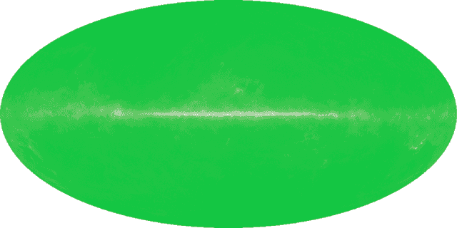
Fig 1. The cosmic microwave background is seen by the Bell Labs Holmdel Horn Antenna in 1965. The solid green represents the uniform $3.5 \pm 1\, {\rm K}$ radiation. The Milky Way is the white strip across the center.

Experimental confirmation of the “near-perfect blackbody” claim wouldn’t come for another 25 years. NASA’s Cosmic Background Explorer (COBE) launched in late 1989 and got to work measuring the spectrum of CMB photons in the wavelength range $2$ to $21\, {\rm cm}$. Within the first year, data from COBE’s Far Infrared Absolute Spectrophotometer (FIRAS) had already begun to reveal a spectrum lying within 1% of a $2.735 \pm 0.06\, {\rm K}$ blackbody [3]. The COBE team later refined this result to conclude a near-perfect blackbody spectrum with a temperature to $2.728 \pm 0.004\, {\rm K}$[4], providing one of the best-traveled experimental visualizations in the history of cosmology,

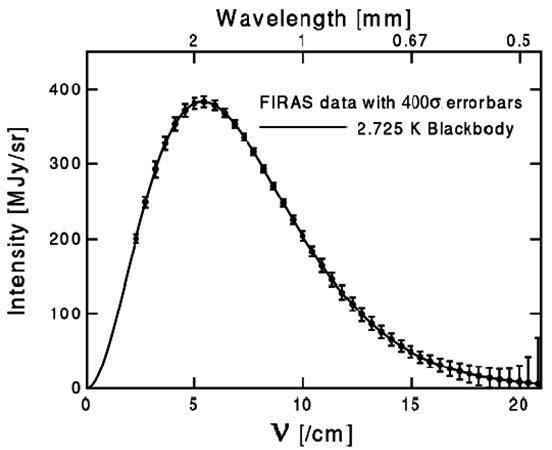
Fig 2. Frequency vs. intensity of the CMB. This figure exists in 85% of all CMB presentations. If the presenter carefully delivers the “curve is thicker than the error bars” line, hushed snickers occur in 100% of cases.

The error bars correspond to an obnoxious $400$ standard deviations, $\sigma$. Why $400\sigma$? Because the more well-mannered $3$, $4$, or $5\sigma$ errors are too small to be seen against the thickness of the line making up the theoretical blackbody curve. File this under “superb and insanely exquisite experimental confirmation of deep and profound theoretical result.” It’s truly impressive.

The COBE satellite was equipped with more than just the FIRAS instrument. A second major objective of the COBE mission was to challenge the near-perfect isotropy of the CMB temperature initially reported by Penzias and Wilson. COBE carefully studied the CMB with its Differential Microwave Radiometer (DMR), hunting for temperature differences between points in the sky separated by $60^\circ$. COBE scanned the entire sky with a resolution of $7^\circ$, amassing highly redundant measurements of each point compared to all others. The results were truly astounding: a $7\sigma$ detection of a tiny anisotropy at the level of $\Delta T/T_0 = 11 \times 10^{-6}$ [5],

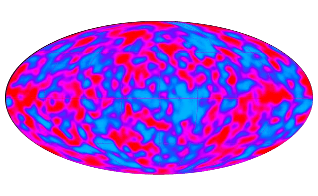
Fig 3. CMB temperature anisotropies exist at a level of one part in $10^5$. This map has been processed to remove galactic sources and something called the CMB dipole, which we’ll talk about shortly. It has a $10^\circ$ resolution. COBE satellite, 1992.

The anisotropy is caused by fluctuations in the temperature of the CMB, leading to direction-dependent temperature variations on the surface of last scattering, $\Delta T(\theta, \phi) = T(\theta, \phi) – T_0$, where $\theta$ and $\phi$ are the usual spherical coordinates. So while COBE FIRAS confirmed that the spectrum of the CMB at each point is a blackbody, the DMR revealed that different points are at slightly different temperatures: the CMB, it seems, is not composed of one, but many ever-so-slightly different blackbodies. That the CMB turned out to be slightly bumpy rather than perfectly smooth has had truly far-reaching consequences for cosmology: the DMR discovery quite literally put cosmology on the map as a precise observational science.

Fast forward to the 21st century, through a decade of ground-breaking science by COBE’s successor, the NASA Wilkinson Microwave Anisotropy Probe (WMAP), designed to map the minute temperature fluctuations discovered by COBE at much higher resolution. As we’ll discuss, CMB data from WMAP was our first real acquaintance with the universe: for the first time, we were able to accurately determine its age, its geometry, and its content. WMAP passed the torch to the European Space Agency’s Planck Surveyor satellite in 2013, which set yet another gold standard with a resolution two orders of magnitude better than COBE. Here is Planck‘s view of the cosmos:

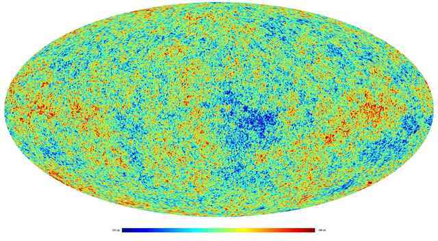
Fig 4. The cosmic microwave background as seen (after processing) by the European Space Agency’s Planck satellite, 2013.

The temperature fluctuations in Figures 3 and 4 look random, like a disordered and haphazard smattering of cold blue and hot red spots. Indeed, the amplitudes of the fluctuations are random—Gaussian as far as we can tell⁴. But that’s not to say that there isn’t information buried in this mess. For example, the Earth moves relative to the CMB at a speed of $370\, {\rm km/s}$ and so the CMB should appear Doppler-shifted: hotter in the direction of motion and colder aft. In other words, we should expect to see one half of Figure 4 redshifted (generally bluer) relative to the other half⁵. Do you see it? I don’t think you can—it’s covered by a blanket of smaller-scale temperature fluctuations. How might we extract it?

Consider the following curve:

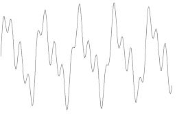
Fig 5. Funky Waveform

What do you make of it? It appears periodic, except that the shape of each cycle is slightly different from the one before it. Thanks to Jean-Baptiste Joseph Fourier, an 18th-century French mathematician with a very French name, we have a way of analyzing this waveform. Fourier showed that any arbitrary periodic function can be remarkably decomposed into a collection of sines and cosines,
$$f(x) = a_0 + \sum_{n=1}^\infty a_n \cos (nx) + \sum_{n=1}^\infty b_n \sin (nx).$$
The secret sauce underwriting the method is the orthogonality of the basis functions, the sinusoids: just as an arbitrary vector can be understood as multiples of its bases, so too, apparently, can certain classes of function be built from orthogonal elements. Writing the funky waveform in Figure 5 as a Fourier series reveals it to be the superposition of three sine functions with different periods and amplitudes,

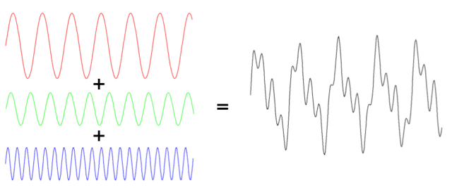
Fig 6. Fourier decomposition of the funky waveform of Figure 5.

Although it might not look it, this simple exercise in the Fourier series is highly relevant to our ability to analyze the CMB temperature maps because it enables us to separate out signals on different scales. Only one problem: Fourier analysis works in flat space, whereas we’re dealing with the surface of a sphere—the surface of the last scattering. It turns out that there is a breed of orthogonal function that lives on the sphere: the spherical harmonics, $Y_{\ell m}$, which are solutions to the angular part of Laplace’s equation in three-dimensional spherical coordinates. They are separable functions of the polar and azimuthal angles, $Y_{\ell m}(\theta, \phi) \propto P_{\ell m}(\cos \theta) e^{im\phi}$, where $P_{\ell m}$ is an associated Legendre function⁶. Notice the two indices: $\ell$ and $m$, necessary for parameterizing the 2-dimensional surface of the sphere. In contrast, the Fourier basis functions live on the 1-dimensional circle (they are periodic on the real line) and so are indexed by a single parameter, $n$, that determines the wavelength of the sinusoid. Varying $\ell$ and $m$ leads to a motley assortment of harmonic functions, Figure 7. For each $\ell$, $m$ takes on values $|m| \leq \ell$.

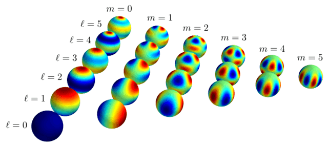
Fig 7. The first few spherical harmonics, parameterized by $\ell$ and $m$. Figures 7, 8, and 9 created with the nifty python script found here.

The role of $\ell$ and $m$ in the functional form of the spherical harmonics—the patterns of blue and red regions on the spherical surface—is less clear than the role of $n$ in the Fourier basis functions. We can gain some insight by studying just the $m=0$ (so-called zonal) harmonics,

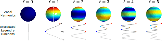
Fig 8. The first few zonal ($m=0$) harmonics. The graphs underneath are the $P_{\ell 0}(\cos \theta)$ illustrating the $\theta$-dependence of the $Y_{\ell 0}$; in particular, the frequency of the $Y_{\ell 0}$ is $\ell$.  The curves are turned on their sides (rotated $90^\circ$ clockwise) for the sake of illustration. The grayed out portions of the curves describe the backside of the harmonics.

The zonal harmonics carry no $\phi$-dependence (they are rotationally symmetric in the azimuthal direction), their $\theta$-dependence being completely determined by the Legendre functions, $Y_{\ell m}(\theta) \propto P_{\ell m}(\cos \theta)$, pictured below the harmonics. The Legendre functions are shown on the domain $[0,2\pi]$, describing one full trip around the spherical harmonic in the longitudinal direction. Using $\ell = 1$ as an example, the hot and cold regions of the harmonic are separated by an angle of $\vartheta_1 = \Delta \theta = \theta_{\rm H} – \theta_{\rm C} = \pi$, with the hot region at the peak of the Legendre function, $\theta_{\rm H} = 0 = 2\pi$, and the cold region at the trough, $\theta_{\rm C} = \pi$, and so we complete one full period as we go once around the surface of the sphere. For $\ell =2$, the hot and cold regions are separated by $\vartheta_2 = \pi/2$, for $\ell = 3$ by $\vartheta_3 = \pi/3$, and in general, $\vartheta_\ell = \pi/\ell$. The zonal harmonics motivate an interpretation of $\ell$ as the frequency of the spherical harmonic.

The index $m$, meanwhile, determines how the hot and cold spots are distributed in the azimuthal direction. Take a look at Figure 9 which shows the $\ell = 5$ harmonics, top view first.

 

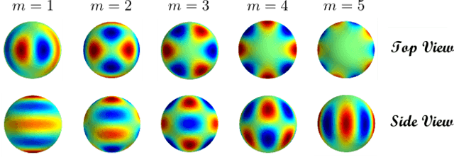
Fig. 9 $\ell = 5$ harmonics, top and side views.

As $m$ increases, the number of pairs of hot and cold regions traversed in the azimuthal direction grows. It too is a frequency, $Y_{\ell m} \propto e^{im\phi}$: for $m=1$, there is a single pair of hot and cold regions, giving a frequency of $m=1$ in the $\phi$ direction. For $m=2$, there are two pairs, and so on. Interestingly, the side view shows us that as $m$ increases, the frequency in the $\theta$-direction decreases: for $m=1$, the frequency in the $\theta$-direction is 5, for $m=2$ it is 4, and in general, it is $\ell – m + 1$ for $m>0$. In other words, the frequency can grow in the $\phi$-direction only at the “expense” of the frequency in the $\theta$-direction. This confirms the view that the overall frequency of the harmonic is set by $\ell$, while $m$ determines how it is distributed.

Getting back to the CMB, the idea is to write the temperature fluctuation as a function of $\theta$ and $\phi$ on the last scattering sphere in terms of the spherical harmonics,
$$\frac{\Delta T}{T_0}(\theta, \phi) = \sum_{\ell, m} a_{\ell m} Y_{\ell m}(\theta, \phi),$$
where the $a_{\ell m}$ are (generally complex) amplitudes and $T$ is the average CMB temperature. This is sometimes called a multipole expansion, in recognition of the role of the $Y_{\ell m}$ in describing multipolar distributions. For example, the $\ell = 1$ harmonics are the basis functions necessary for describing the electric potential of a dipole, the $\ell = 2$ harmonics give the potential of a quadrupole, and so on. Just like Fourier analysis, the expansion in terms of spherical harmonics permits us to study the contributions to the CMB coming from temperature fluctuations existing on different scales. On the surface of the sphere, these are angular scales $\vartheta_\ell = \pi/\ell$. Consider the CMB dipole term: $\Delta T/T_0|_{\rm dipole} = \sum_{m} a_{1 m} Y_{1 m} = \sqrt{3/8\pi}\cos(\phi)\sin(\theta)(a_{1 -1} – a_{1 1}) + \sqrt{3/4\pi}a_{10}\cos(\theta)$, which describes a hot and a cold spot separated by $\vartheta = 180^\circ$. With the z-axis taken in the direction of the Earth’s motion, the dipole is dominated by $Y_{10}$. This is precisely the effect we were earlier hoping to extract from the complete CMB maps: it arises as a result of the Earth’s motion relative to the CMB. COBE was the first probe to measure the dipole anisotropy, with $\Delta T/T_0|_{\rm dipole} = 3.353 \pm 0.024\, {\rm mK}$ [6] (later tightened slightly by WMAP to $3.346 \pm 0.017\, {\rm mK}$ [7]),

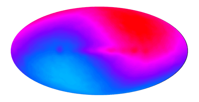
Fig 10. CMB dipole anisotropy as measured by COBE. Evidence that Copernicus was right.

Assuming that the dipole anisotropy is largely due to Earth’s motion (a safe assumption, as we’ll come to see), the velocity of the Earth relative to the CMB can be found by writing the Doppler shift in terms of temperature via Planck’s law [8], giving a velocity of $v = 368 \pm 2\, {\rm km/s}$ towards galactic coordinates $(l, b) = (263.85^\circ \pm 0.10^\circ, 48.25^\circ \pm 0.04^\circ)$ [7]. Pretty cool. And that’s just a taste of what we can learn from the CMB anisotropies.

But why stop at the dipole? Figure 11 depicts the $\ell =2,\, 3,$ and $4$ multipole moments. Each of these maps is a linear combination of the spherical harmonics with $|m| \leq \ell$ projected onto the plane. Notice that the quadrupole map is noticeably cooler than the others, indicating that fluctuations on different scales have different amplitudes.

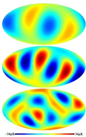
Fig 11. CMB quadrupole, octupole, and hexadecapole from WMAP. Figure from [9].

To determine the amplitudes of each multipole moment, naively we might think to average the $a_{\ell m}$’s at each $\ell$; however, of course $\langle a_{\ell m}\rangle = 0$. This is true by definition: the $a_{\ell m}$’s parameterize deviations from the average CMB temperature, so of course their average must vanish. Instead, we want something like a squared deviation—a variance—of the $a_{\ell m}$’s which we don’t expect will vanish. To compute the variance, we need two points on the last scattering surface, $(\theta,\phi)$ and $(\theta’,\phi’)$, in the direction of unit vectors ${\bf n}$ and ${\bf n’}$ separated by an angle $\vartheta = \cos^{-1}({\bf n}\cdot{\bf n’})$. Record the temperature of the CMB at the two locations to obtain $\Delta T({\bf n})/T_0$ and $\Delta T({\bf n’})/T_0$. Repeat this measurement across the entire last scattering surface, for all pairs of points separated by the angle $\vartheta$, and take the average over all pairs,
$$\left\langle\frac{\Delta T({\bf n})}{T_0}\frac{\Delta T({\bf n’})}{T_0}\right\rangle = \sum_{\ell m}\sum_{\ell’ m’}\langle a^*_{\ell m}a_{\ell’ m’}\rangle Y^*_{\ell m}(\theta, \phi)Y_{\ell’ m’}(\theta’, \phi’) = \sum_\ell \left(\frac{2\ell + 1}{4\pi}\right)C_\ell P_\ell({\bf n}\cdot{\bf n’}),$$
where the second line follows from the spherical harmonic addition theorem, the $P_\ell({\bf n}\cdot{\bf n’}) = P_\ell(\cos \vartheta)$ are the Legendre polynomials, and
$$\langle a^*_{\ell m} a_{\ell’ m’}\rangle = \delta_{\ell \ell’}\delta_{m m’}C_\ell.$$
There’s a lot going on in the above equations, so let’s walk through them carefully. First, the individual $a_{\ell m}$’s are Gaussian-distributed random variables⁷ with mean zero, as discussed. Via Eq. (4), the temperature fluctuation $\Delta T({\bf n})$ is also then a Gaussian-distributed random variable with mean zero, $\langle \Delta T({\bf n}) \rangle = 0$. The quantity $C_\ell$ is what we are after: it is the variance of the $a_{\ell m}$’s for each $\ell$, giving a measure of the average squared amplitude of each multipole moment. The universe is generally believed to be statistically isotropic—the flucutations do not favor one region of the last scattering surface over any other—and so the variance does not depend on $m$ (which, if you recall, is in charge of distributing the fluctuations around the sphere.) Meanwhile, the Legendre functions, $P_\ell (\cos \vartheta)$, determine the degree to which the different multipole moments contribute to fluctuations on angular scale $\vartheta$: the multipole moment of order $\ell$ contributes most strongly to fluctuations on angular scales⁸$\vartheta_\ell \approx \pi/\ell$ (the Legendre function of order $\ell$ has an extremum near $\vartheta_\ell = \pi/\ell$), but each multipole contributes to fluctuations on all angular scales (except where $P_\ell (\cos \vartheta) = 0$). For example, the multipole moment of order $\ell$ provides a near-constant contribution to fluctuations on much smaller scales $\vartheta \ll \pi/\ell$, and contributes maximally to larger scale fluctuations that are integer multiples of $\vartheta_\ell$.

Figure 12 summarizes the roles of $C_\ell$ and $P_\ell (\cos \vartheta)$:

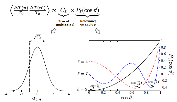
Fig 12. Main ingredients going into $\langle \Delta T({\bf n})/T_0 \cdot \Delta T({\bf n’})/T_0\rangle$. On the left is the distribution of the $a_{\ell m}$’s at fixed $\ell$: $C_\ell$ is the variance of the Gaussian distribution, providing a measure of the amplitude of the $\ell$-order multipole moment. On the right are a few of the low-order Legendre polynomials: these control the degree to which each multipole moment contributes to fluctuations on the scale $\vartheta$. The Legendre polynomial of order $\ell$ contributes most to scales near $\vartheta_\ell = \pi/\ell$.

Taken together and summed over $\ell$, they give the average value of the product of two⁹temperature fluctuations separated by an angle $\vartheta$, which is just what we have written on the left-hand side of Eq. (5). It turns out that the quantity $\langle \Delta T({\bf n})/T_0 \cdot \Delta T({\bf n’})/T_0\rangle$ is a measure of the statistical correlation of the two random fluctuations $\Delta T({\bf n})/T_0$ and $\Delta T({\bf n’})/T_0$. To assess the statistical independence of two random variables, $X$ and $Y$, the expectation values $\langle X \rangle$ and $\langle Y \rangle$ are subtracted from the expectation value of the product of $X$ and $Y$, ${\rm corr}[X,Y] = \langle XY \rangle – \langle X \rangle \langle Y \rangle$. Statistical independence ensures that $\langle XY \rangle = \langle X \rangle \langle Y \rangle$ and indicates zero correlation between $X$ and $Y$. Because $\langle \Delta T({\bf n})\rangle = \langle \Delta T({\bf n’})\rangle = 0$, the correlation of temperature fluctuations is ${\rm corr}[\Delta T({\bf n})/T_0,\Delta T({\bf n’})/T_0] = C(\vartheta) = \langle \Delta T({\bf n})T_0 \cdot \Delta T({\bf n’})/T_0\rangle$. The function $C(\vartheta)$ is referred to as the temperature correlation function, or two-point angular correlation function. The correlation function tells us that collections of points separated by $\vartheta$ are statistically related, and as we’ll come to see, this is because they are physically related.

The $C_\ell$’s contain the same information as the $C(\vartheta)$, but they tell the story of CMB temperature fluctuations in harmonic ($\ell$) space rather than real ($\vartheta$) space. These dual views motivate an appreciation of Eq. (5) as a Legendre transform,
$$C(\vartheta) = \sum_\ell \left(\frac{2\ell + 1}{4\pi}\right)C_\ell P_\ell(\cos \vartheta),$$
which, much like the Fourier transform, facilitates the translation between the harmonic amplitudes and real-space correlations (with the $P_\ell (\cos \vartheta)$ as basis function instead of sinusoids.) In this light, the $C_\ell$’s are often refered to as the temperature power spectrum, or angular power spectrum. We can measure the $C_\ell$’s across a rather impressive range of $\ell$, thanks to modern probes: Planck covers the range $\ell = 2-2500$. When we do, a truly marvelous picture emerges,
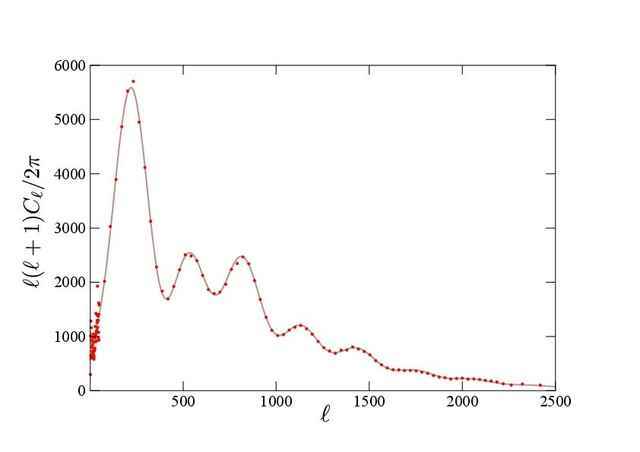Fig 13. Temperature power spectrum data as measured by Planck and best-fit theoretical spectrum. Planck data from http://www.cosmos.esa.int/web/planck.

These are the famous $C_\ell$’s in their full glory. We can also display the $C_\ell$’s in terms of $\vartheta_\ell = \pi/\ell$, the approximate angular scale they most influence, Figure 14. Planck has the resolution to probe angular scales $\vartheta = 90^\circ – 0.07^\circ$.
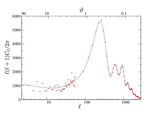Fig 14.Temperature power spectrum as a function of $\vartheta$. Multipole moments of order $\ell$ contribute most strongly to fluctuations on angular scales $\vartheta_\ell = \pi/\ell$. We use a logarithmic scale to display the large angular behavior.

Notice the characteristic wiggles in the spectrum: we know that the dipole is due to the Earth’s motion through space, but what about these mysterious, smaller-scale temperature fluctuations? Unlike the dipole, they are intrinsic to the CMB, in that their source pre-dates the creation of the cosmic background radiation. Because the CMB is largely decoupled from the rest of the universe, these fluctuations are well-preserved fossils of the primordial universe, encoding important information about its thermal history. The undulating correlations in the power spectrum bespeak some causal, ordered process at work in the baryon-photon plasma. In the next note, we’ll explore the physics behind these temperature fluctuations.

Before wrapping up, a word on averages. The angled brackets in the equations above are supposed to denote an average overall observer position (so that we can measure “the thing”, not the “the thing from our perspective.”) As we’ve just seen, however, temperature fluctuations are correlated and so nearby observers will generally observe similar CMB skies. The best way to get independent measurements of uncorrelated fluctuations is to consider observer positions very far apart, say, across the observable universe where spatial coherence is at a minimum. Because such observers effectively measure a different universe, the average $\langle \cdot \rangle$ is sometimes called an ensemble average, meaning it should be taken over an ensemble of different universes. Without some seriously impressive rocketry, this is impossible. The best we can do is compute $\langle |a_{\ell m}|^2\rangle$ by averaging over $m$,
$$C_\ell = \frac{1}{2\ell + 1}\sum_{m=-\ell}^\ell \langle |a_{\ell m}|^2\rangle.$$
Because the contributions to $\Delta T({\bf n})$ from different $m$ are independent, we can get $2\ell + 1$ measurements for each $\ell$ this way. And don’t worry—the average over $m$ is a permissible stand-in for the ensemble average as long as the universe is sufficiently isotropic that observations made from Earth are statistically consistent with observations made from elsewhere in the universes¹⁰. This is the kind of averaging I described in a slightly different language just before Eq. (5). The downside to averaging over $m$ is that for low $\ell$, we get only relatively few measurements: one for each of the $2\ell + 1$ spherical harmonics. The variance, $C_\ell$, is therefore only an estimate of the true variance of the distribution of the $a_{\ell m}$’s. The standard error of any such test statistic goes as $1/\sqrt{N}$, where $N$ is the number of data points, and so the standard error on the estimate of $C_\ell$, $\Delta C_\ell$, can therefore not be improved beyond¹¹
$$\frac{\Delta C_\ell}{C_\ell} = \sqrt{\frac{2}{2\ell + 1}}.$$
This fundamental uncertainty, known as cosmic variance, presents an upper limit on the resolution of the CMB temperature power spectrum: we cannot engineer our way out of it because it is a statistical error arising from the small sample size at low $\ell$. It is often said that cosmic variance is a problem because we only have one universe to look at. This is true, but we shouldn’t despair: there is still plenty we can find out about the universe by looking at the CMB.

References and Footnotes

[1] Dicke, R.H., Peebles, P. J. E., Roll, P. G., Wilkinson, D.T., Cosmic Black-Body Radiation. Astrophysical Journal, 142 (1965).
[2] Penzias, A. A., Wilson, R. W., A Measurement of Excess Antenna Temperature at 4080 Mc/s. Astrophysical Journal, 142 (1965).
[3] Mather, J. C., et al., A preliminary measurement of the Cosmic Microwave Background by the Cosmic Background Explorer (COBE) Satellite. Astrophysical Journal, 354 (1990).
[4] Fixsen, E. S., et al., The Cosmic Microwave Background spectrum from the full COBE FIRAS data set. Astrophysical Journal, 473 (1996).
[5] Smoot, G. F., et al., Structure in the COBE differential microwave radiometer first-year maps. Astrophysical Journal, 396 (1992).
[6] Bennett, C. L., et al., Four-Year COBE DMR Cosmic Microwave Background Observations: Maps and Basic Results. Astrophysical Journal, 464 (1996).
[7] Bennett, C. L., et al., First-Year Wilkinson Microwave Anisotropy Probe (WMAP) Observations: Preliminary Maps and Basic Results. Astrophysical Journal, 148 (2003).
[8] Peebles, P. J. E., Wilkinson, D. T., Comment on the Anisotropy of the Primeval Fireball. Physical Review, 174 (1968).
[9] Tegmark, M., de Oliveira-Costa, A., Hamilton, A., A high resolution foreground cleaned CMB map from WMAP. Physical Review, D68 (2003).

¹The spectrum should be “near” blackbody because various events post-decoupling, including interactions with ionized gas during the epoch of star formation, can lead to deviations from a blackbody spectrum. back
²They assumed a blackbody; experimental confirmation of this would have to await the early 1990’s and NASA’s Cosmic Background Explorer (COBE) satellite. back
³This observation cannot be adequately explained by the standard hot big bang model. A brief period of primordial inflation renders the observable universe homogeneous and isotropic, and is one proposed explanation. back
⁴There are several curious anomalies and suspicious coincidences that appear to violate statistical isotropy and Gaussianity, but apart from these cases there are no statistically significant deviations from a Gaussian random field. I hope to talk about some of this stuff in a later note. back
⁵Recall that maps like Figure 11 are flat projections of the last scattering sphere surrounding Earth. back
⁶Related to the tenured Legendre function by $P_{\ell m}(x) = (-1)^m(1-x^2)^{m/2}\frac{{\rm d}^m}{{\rm d}x^m}P_\ell (x)$. back
⁷This is a basic prediction of inflationary cosmology and is consistent with observations. back
⁸Recall that for the zonal harmonic of order $\ell$, the angular separation of adjacent hot and cold spots is $\vartheta_\ell = \pi/\ell$. This is no longer exactly true when we consider the $Y_{\ell m}$ with $|m|>0$; for example, as one moves around $Y_{54}$ in the $\phi$-direction, hot and cold spots are separated by $\pi/4$, whereas for $Y_{55}$ they are separated by $\pi/5$ (cf. Figure 9). Hence, in what follows we will write $\vartheta_\ell \approx \pi/\ell$. back
⁹Because the $C_\ell$’s are the average squared amplitudes. back
¹⁰Again, this is mostly the case except for a few possible exceptions on the largest length scales. back
¹¹We arrive at this expression as follows. First, note that the $C_\ell$’s are the estimated variance of the measured $a_{\ell m}$’s. If we could calculate $C_\ell$ for a given $\ell$ across independent observing locations (equivalently, across many different universes), then we expect $\langle C_\ell \rangle = C_\ell^{\rm true}$—that the mean of this collection of $C_\ell$’s, each describing a different sample from the true distribution of the $a_{\ell m}$’s, should converge to the true variance of this distribution, $C_\ell^{\rm true}$, as the number of measurements grows. We’d like to understand the uncertainty in our estimate of $C_\ell$, $\Delta C_\ell$, given that we have so few measurements (only $2\ell + 1$) for each $\ell$. Now, the $a_{\ell m}$’s are Gaussian random variables, which means they are drawn from a distribution $\sim \exp\left(a_{\ell m}/\sqrt{C_\ell^{\rm true}}\right)$, where $C_\ell^{\rm true}$ is the variance of the true distribution. Because $C_\ell^{\rm true}$ is a constant, the quantity $a_{\ell m}/\sqrt{C_\ell^{\rm true}}$ is likewise Gaussian-distributed. Then, note that the quantity
$$V_\ell = \frac{1}{C_\ell^{\rm true}}\sum_{m = -\ell}^\ell |a_{\ell m}|^2 = (2\ell+1)\frac{C_\ell}{C_\ell^{\rm true}},$$
as the sum of the squares of Gaussian random variables, is $\chi^2_\nu$-distributed with $\nu = 2\ell + 1$ degrees of freedom. The variance of a $\chi^2_\nu$-distributed random variable is $2\nu$, and so we write
$$(\Delta V_\ell)^2 = 2(2\ell+1) = (2\ell + 1)^2\left(\frac{\Delta C_\ell}{C_\ell^{\rm true}}\right)^2,$$
giving
$$\frac{\Delta C_\ell}{C_\ell} = \sqrt{\frac{2}{2\ell+1}}.$$ back

Click For Forum Comments