A Poor Man’s CMB Primer: Quantum Seeds

 

The CMB establishes a record of ancient acoustic oscillations in the baryon-photon plasma. We’ve been studying how these primordial sound waves evolve, and how to analyze the last scattering surface to learn about them. Now it’s time to confront their origin: what process composed the cosmic symphony? A few different proposals have been advanced over the years to explain the origin of the primordial perturbations. Thermal fluctuations and topological defects have been investigated; the latter is ruled out by current CMB data, while the former provides for a viable mechanism in string gas and contracting universe models. By far the most remarkable story, though, has it that large-scale structure is actually of quantum mechanical origin—that the density perturbations are amplified and frozen quantum fluctuations. This bizarre proposal is realized in the inflationary universe scenario, in which a brief but decisive period of exponential expansion stretched the universe from its primordial infancy to at least its present size. As we’ll explore in this section, this stretching succeeded in magnifying and preserving the quantum jitters of the fields permeating space; in the post-inflationary universe, these fluctuations are found to source density perturbations of a kind in near-perfect accord with CMB observations.

To get a handle on the dynamics, consider the second time derivative of the Friedmann equation, $H^2 = 8\pi G \rho/3$, together with the continuity equation, $\dot{\rho} = -3H(\rho + p)$,
\begin{equation}
\label{FE2}
\frac{\ddot{a}}{a} = -\frac{4\pi G}{3} \left(\rho + 3p \right).
\end{equation}
This equation relates the rate of change of the scale factor, $a(t)$, to the trace of the stress-energy tensor, $T^\mu{}_\mu = \rho – 3p$. Notice that if $p < -\rho/3$, the universe undergoes accelerated expansion. Accelerated expansion is referred to as inflation.

Consider next a scalar field uniformly distributed across space with energy density and pressure,
\begin{eqnarray}
\label{dp}
\rho &=& \frac{1}{2}\dot{\phi}^2 + V(\phi), \nonumber \\
p &=& \frac{1}{2}\dot{\phi}^2 – V(\phi).
\end{eqnarray}
If we assume that the scalar field has very little kinetic as compared to potential energy, $\dot{\phi}^2/2 \ll V(\phi)$, then $p \approx -\rho$ and, as per Eq. (\ref{FE2}), the condition for accelerated expansion is satisfied. If we imagine that $V(\phi)$ is a monotonically decreasing function of $\phi$, then as the field evolves potential energy is converted to kinetic, just like a classical ball rolling down a hill. Eventually, if the kinetic energy grows beyond the value $2V(\phi)$, the scale factor no longer accelerates, and the universe stops inflating (again, as per Eq. (\ref{FE2})). We have then, via the scalar field, a simple mechanism for initiating a period of inflation, and then bringing it to a close. Inflation doesn’t need to last very long to cause some serious expansion: that’s because the scale factor grows near-exponentially, $a(t) \approx e^{Ht}$ with $H^2 \approx V \approx const$, when $\dot{\phi}^2/2 \ll V$. Indeed, inflationary expansion caused at least an $e^{60}$-fold increase in the scale factor in less than $\Delta t \approx 10^{-34}$ seconds (assuming $H$ is near the grand unification scale.) Such tremendous expansion leaves the universe very smooth, very cold, and very empty (e.g. matter densities are diluted by a factor of $e^{180}$). So what, then, of the CMB? Shouldn’t inflation have erased it?

Though we don’t know what field drove inflation, it is generally expected that this field—inflation—should find a home in some extension of the standard model of particle physics, and it should interact with some of the particle species in this theory. When the inflation attains its minimum potential energy, it condenses into a sea of particles as the field executes oscillations about this minimum (glance ahead to Figure 2 for help visualizing this.) The inflation particles are massive, and the universe is cold, and so the inflation soon decays into those particles with which it interacts according to the prevailing particle physics model. This decay process reheats the universe into a hot, radiation-dominated phase identical to that expected following the Big Bang. The radiation that results from the inflaton decay goes on to make up the CMB. And so, operationally, the end of inflation can be taken to coincide with the standard Big Bang, insofar as it sets up identical initial conditions for the subsequent standard cosmological evolution. What of the “true” big bang before inflation? Nobody knows.  Figure 1 is a popular depiction of this timeline, compliments of NASA, with inflation placed before the generation of the CMB and after the mysterious origin of the universe.

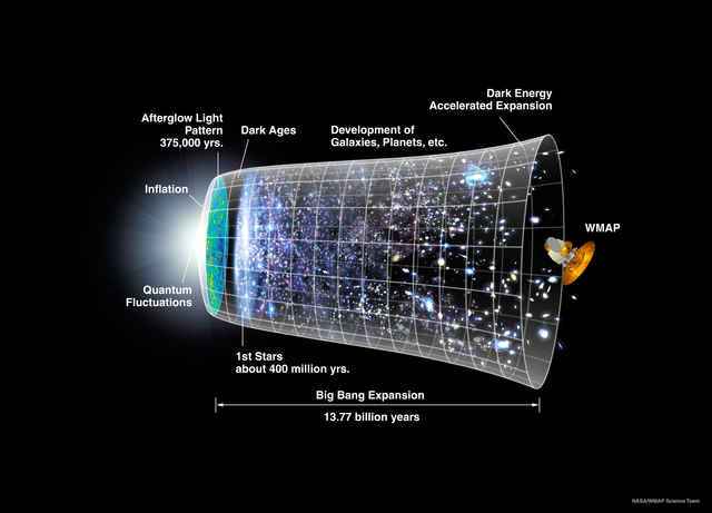
Fig 1. Chronology of the universe. Image credit NASA/WMAP Science Team, 2006.

Whatever the true identity of inflation, we know it must be a quantum field. This means, among other things, that we cannot be certain of its value at a given point in spacetime, $\phi(x)$. In particular, the function $\phi({\bf x})$ at a particular instant in time will vary from place to place. Dynamically, we understand this as follows: while the classical motion of the inflation flows strictly from high to low potential energy, as it “rolls down” the potential energy function there is some fuzziness to its actual trajectory,

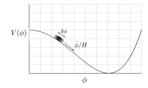
Fig 2. Classical rolling of the inflation, with quantum fluctuations, superposed on the classical motion.

Quantum jitters cause the field to take small, discrete hops up or down the potential, resulting in small variations in field energy across space.

At any particular instant in time, space looks like the illustration in Figure 3, which is a random superposition of separate inflating regions; each inflating region is caused by a fluctuation of the inflation field about the average density:

Fig 3. The energy of the inflation field across space at an instant in time. Variations arise as random fluctuations, each leading to a separate inflating region of space. The image is a still frame from the animated gif found at http://www.astro.ucla.edu/~wright/CMB-MN-03/epas.html

Once a fluctuation occurs somewhere in space, that region undergoes inflation according to the classical energy density there; after a time, this inflating region might give rise to more fluctuations. At any instant in time, these later fluctuation events appear as smaller inflating regions within the larger, earlier-nucleated regions.

The result of all this is that different parts of the universe will end inflation at different times. The reason is easy to see: as the classical motion of the field approaches the point along with the potential at which the inflationary condition ceases to hold, quantum fluctuations might kick the field further down the potential in one place, ending inflation there, while somewhere else a fluctuation might send the field back up the potential, nucleating new inflationary regions. Eventually, inflation comes to an end, albeit at different times, across a region of space roughly the size of today’s Hubble sphere. Those places that ended inflation earlier reheated sooner, undergoing non-inflationary expansion for longer: the result is a bumpy energy landscape across space at the end of inflation.

To examine the behavior of perturbations on individual length scales, we employ the Fourier transform to write the spatial density contrast field in terms of its components,
\begin{equation}
\label{f2}
\delta ({\bf x},t) = \int \frac{{\rm d}^3 k}{(2\pi)^{3/2}}\delta_k(t) e^{-i{\bf k}\cdot{\bf r}},
\end{equation}
where recall that ${\bf k}$ and ${\bf r}$ are comoving quantities. The scale, $k$, of a fluctuation region at the time it stops inflating is determined, simply, by how long it inflated for, $\Delta t = t_{\rm end} – t_i$. Meanwhile, the amplitude of the fluctuation is determined by the length of time it undergoes non-inflationary expansion relative to other regions in the Hubble patch, $\delta t$. Consider a region of the universe that stopped inflating a time $\delta t$ sooner than another region. According to the continuity equation, the difference in density is proportional to this time shift,
\begin{equation}
\label{dt}
\frac{\delta \rho}{\bar{\rho}} = \delta = cH\delta t,
\end{equation}
where the constant $c$ is determined by the dominant form of energy after inflation¹. Notice that it’s possible to have perturbations on the same scale with different amplitudes. Take a look at Figure 4:

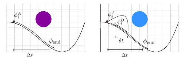
Fig 4. Fluctuation regions on the same length scale with different amplitudes.

Imagine region $A$ undergoes inflation with an initial field value, $\phi^A_{i}$, high-up on the potential as shown.
Suppose it rolls down to $\phi_{\rm end}$ in time $\Delta t$. Another region, $B$, starts inflating at the same time as region $A$ but at a slightly lower energy density: after the field rolls down classically for a time, $\delta t$, there is a quantum jump up to $\phi^A_{i}$. This nucleates a fluctuation region that begins to inflate from $\phi^A_{i}$, and so, like region $A$, rolls down to $\phi_{\rm end}$ in time $\Delta t$. Both region A and the fluctuation within region $B$ are the same size since they both inflated for a time $\Delta t$, however, region $A$ ended inflation a time $\delta t$ sooner, and, hence, has a different density.

Of particular interest is how great this variability in density is as a function of scale. The variance of the energy density about the mean on a length scale given by comoving wavenumber, $k$, is written
\begin{equation}
\label{var}
\langle |\delta_k |^2 \rangle = c^2H^2 \delta t^2 \propto \underbrace{\left(\frac{H}{\dot{\phi}}\right)^2}_\text{ classical}\underbrace{\langle |\delta \phi_k|^2\rangle}_\text{quantum},
\end{equation}
where we’ve made explicit contributions from the classical rolling and the quantum jumping of the field. The quantum contribution to the variance is at present quite mysterious; however, since $H$ is very nearly constant, the contribution of the classical evolution to the scale-dependence of the variance is evidently through $\dot{\phi}$. Why is this? Look back at Figure 4: suppose that $\phi$ is moving initially very slowly as it begins to roll down the potential. The more slowly the field traverses a given range $\Delta \phi$, the more “opportunities” it has to make a quantum jump to new field values within the range $\langle \delta \phi_k \rangle$. As Figure 4 illustrates, when a certain field value is reached via quantum fluctuation at different times in different parts of the universe, the regions have different post-inflationary energy densities. Hence, when $\dot{\phi}$ is small relative to the expansion rate, $H$, there is high variability in the perturbation amplitudes on a given scale, $k$. In potentials of the type illustrated in Figure 4, $\dot{\phi}$ increases with time and so we expect higher variability on large length scales (small $k$ and small $\phi_k$) than small length scales (larger $k$ and larger $\phi_k$). This kind of perturbation spectrum is called a red spectrum because there is more power (variability) on large-length scales (or infrared momenta, $k$). Conversely, if $\dot{\phi}$ is initially large and decreasing, we expect the reverse: more opportunities to nucleate regions down towards the bottom of the potential. This spectrum is blue because there’s more power on small-length scales (or ultraviolet momenta, $k$).  Figure 5 is an illustration of a red spectrum:

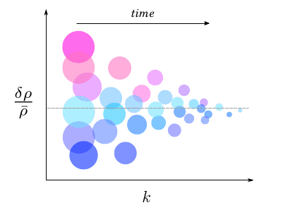
Fig 5. Cartoon of how the densities of fluctuations vary with scale. This is an example of a “red” spectrum, with greater variability on large length scales (small $k$). Don’t put any thought into the shape of the tapering: this is merely an illustration!

So we’ve seen how the classical dynamics of the inflation field, exhibited through the quantity $H/\dot{\phi}$, determines the scale dependence of the perturbation spectrum. Now let’s explore the role of the quantum fluctuation amplitude, $\delta \phi_k$. We begin with the equation of motion of the inflation,
\begin{equation}
\label{KGE}
\ddot{\phi} + 3H \dot{\phi} – \frac{\nabla^2}{a^2}\phi + \frac{{\rm d}V(\phi)}{{\rm d}\phi} = 0,
\end{equation}
obtained by dropping the expressions for the energy density and pressure of the scalar field⁴,
\begin{eqnarray}
\rho &=& \frac{1}{2}\dot{\phi}^2 +\frac{1}{2}\frac{\nabla^2}{a^2}\phi+ V(\phi), \nonumber \\
p &=& \frac{1}{2}\dot{\phi}^2 – \frac{1}{6}\frac{\nabla^2}{a^2}\phi- V(\phi),
\end{eqnarray}
into the continuity equation, $\dot{\rho} = 3H(\rho + p)$. We write the field $\phi({\bf x},t) = \phi_0(t) + \delta \phi({\bf x},t)$, where $\phi_0(t)$ is the homogeneous “background” field value, and the perturbations are taken to be small relative to it, $\delta \phi({\bf x},t) \ll \phi_0(t)$. To first order in $\delta \phi$, Eq. (\ref{KGE}) becomes
\begin{equation}
\label{fluceq}
\ddot{\delta \phi} + 3H\dot{\delta \phi} -\left(\frac{\nabla^2}{a^2} – \left.\frac{{\rm d}^2V(\phi)}{{\rm d}\phi^2}\right|_{\phi = \phi_0}\right)\delta \phi = 0,
\end{equation}
where the second derivative of $V(\phi)$ appears because we’ve expanded $\left.\frac{{\rm d}}{{\rm d}\phi}V(\phi)\right|_{\phi = \phi_0 + \delta \phi}$ about $\phi_0$, chosen to be a local minimum of $V(\phi)$, and keeping terms first-order in $\delta \phi$. In what follows, we assume that $\frac{{\rm d}^2}{{\rm d}\phi^2}V(\phi_0) \approx 0$, since we expect the inflaton potential to be quite flat across scales of interest². Next, we write the Fourier transform of the fluctuation³,
\begin{equation}
\delta \phi({\bf x},t) = \int\frac{{\rm d}^3k}{(2\pi)^{3/2}}\delta \phi_k(t)e^{i{\bf k}\cdot{\bf r}},
\end{equation}
and use it in Eq. (\ref{fluceq}) to obtain
\begin{equation}
\label{premode}
\ddot{\delta \phi_k} + 3H\dot{\delta \phi_k} + \left(\frac{k}{a}\right)^2\delta \phi_k = 0.
\end{equation}
Sadly, there is no analytic solution to this equation for general spacetimes; however, $\delta \phi$ evolves identically in all spacetimes in two distinct limits: very small and very large scales. Let’s pull out a factor of $H^2$ from the last two terms so that we can write
\begin{equation}
\label{kah}
\ddot{\delta \phi_k} + H^2\left[3\frac{\dot{\delta \phi_k}}{H} + \left(\frac{k}{aH}\right)^2\delta \phi_k\right] = 0,
\end{equation}
and consider the term $(k/aH)^2$. During inflation, the size of the cosmological horizon is approximately the Hubble scale, $d_H \sim H^{-1}$, and the physical wavelength of a fluctuation is $\lambda_{\rm phys} = 2\pi a/k$. The quantity $k/aH \sim d_H/\lambda_{\rm phys}$ therefore gives the size of the fluctuation relative to the cosmological horizon, the distance across which causal processes have had time to act since the big bang. To study the evolution of $\delta \phi$ on very small length scales for which $k/aH \gg 1$ dominates the square brackets in Eq. (\ref{kah}), we must solve
\begin{equation}
\ddot{\delta \phi_k} + \left(\frac{k}{a}\right)^2\delta \phi_k = 0.
\end{equation}
This should look familiar! It’s a wave equation in terms of physical wavenumber, $k/a$, with solution $\delta \phi_k \sim \exp(ikt/a)$. Aside from the redshift, exhibited as an increase in wavelength of the fluctuation over time, the inflationary expansion does not affect the evolution of $\delta \phi$. But this makes sense: the frequency of these high-energy fluctuations, $\omega = k/a$, is much greater than the expansion time scale governed by $H$ (remember, $k/aH \gg 1$), and so the fluctuations simply don’t “feel” the expansion. In this limit, fluctuations exhibit wave-like behavior much as they would in static space.

Consider now the opposite extreme: very large wavelength fluctuations, with $k/aH \ll 1$. In Eq. (\ref{kah}), now the first term in the square brackets dominates, with the solution $\delta \phi_k \sim const.$. No longer a wave! This, too, makes intuitive sense: we’re talking about a fluctuation with a physical wavelength larger than the horizon. So, essentially, a single Fourier mode is stretched to length scales surpassing the distance that light could have traveled since the Big Bang. The only expectation, in this case, is that causal dynamics shut off—the mode no longer evolves. So vacuum fluctuations born at small wavelengths initially exhibit wave-like behavior, but after a time they grow too big and “freeze” on superhorizon scales. What do we think is happening in between these asymptotic regimes? If only we had an analytic solution covering the entire evolution of the mode! While we might not have a general solution to Eq. (\ref{premode}), there is an exact solution for one special kind of inflation: true exponential expansion.

Inflation with $H = const.$, known as de Sitter expansion, is exactly exponential, $a(t) \propto e^{Ht}$. Inflation in the real universe could not have been truly de Sitter, or else it would never have ended; however, we expect that inflation was quite close to de Sitter across scales of cosmological interest, and so the quantum fluctuations which can be solved exactly, in this case, serve as a valuable prototype. Before we get there, though, two pieces of housekeeping: let’s change from coordinate to conformal time, ${\rm d} \tau = {\rm d}t/a$; this is a clock that slows down with the expansion of the universe—and rescale the field fluctuation, $u_k = a\delta \phi_k$. This brings us to a neatly compact version of Eq. (\ref{premode}), called the mode equation,
\begin{equation}
\label{modeq}
u_k” + \left(k^2 – \frac{a”}{a}\right)u_k = 0,
\end{equation}
where primes denote derivatives concerning conformal time. The nice thing about the mode equation is that all the cosmological dynamics are neatly packaged up into the $a”/a$ term. Specializing to de Sitter expansion, the conformal time is,
\begin{equation}
\tau = \int {\rm d}t e^{-Ht} = -\frac{1}{aH},
\end{equation}
giving $a(\tau) = -1/(H\tau)$. Notice that $\tau$ is negative during inflation, and we’ve chosen $\tau = 0$ to coincide with the end of inflation. The $a”/a$ term in Eq. (\ref{modeq}) becomes
$$
\frac{a”}{a} = 2a^2H^2 = \frac{2}{\tau^2}
$$
and we can write the mode equation as
$$
(k\tau)^2\frac{{\rm d}^2u_k}{{\rm d}(k\tau)^2} + \left[(k\tau)^2 – 2\right]u_k = 0.
$$
This equation can be solved exactly in terms of Hankel functions,
$$
u_k(-k\tau) = \frac{1}{2}\sqrt{-k \tau}\left[c_1 H^{(1)}_{3/2}(-k\tau) + c_2H^{(2)}_{3/2}(-k\tau)\right],
$$
where $H^{(1)}_{3/2} = J_{3/2} +iY_{3/2} = H^{(2)*}_{3/2}$, and $J_{3/2}$ and $Y_{3/2}$ are Bessel functions of the first and second kind. To determine the coefficients $c_1$ and $c_2$, we appeal to boundary conditions on $u_k(-k\tau)$ and $u’_k(-k\tau)$. We just observed that at very short wavelengths, $k/aH = -k\tau \rightarrow \infty$, the mode $u_k(-k\tau)$ evolves as a plane wave. We can use this fact to get rid of one of the constants. Bessel functions indeed reduce to sinusoids for large arguments, with an asymptotic solution
$$
u_k(-k\tau) = \frac{1}{\sqrt{2k}}\left(c_1 e^{-ik\tau} + c_2 e^{ik\tau}\right).
$$
Matching this solution to that of Eq. (\ref{kah}) requires that “negative” frequency mode not play a role, and so $c_2 = 0$. Next, the coefficient $c_1$ is found by imposing a condition on the first derivative of the mode function, $u_k’$. What do we know about it? In quantum field theory the field operator⁵, here given by $\delta \phi({\bf x},t)$, satisfies a canonical commutation relation, $[\delta \phi({\bf x},\tau),\pi({\bf x}’,\tau’)]_{\tau = \tau’} = i\delta^3({\bf x} – {\bf x}’)$, with a quantity called the conjugate momentum, $\pi({\bf x},t) = a^2\delta \phi({\bf x},t)’$. This commutator is the field-theoretic analog of the Heisenberg uncertainty principle and amounts to a locality constraint on the field operator: the Dirac delta function, $\delta^3({\bf x} – {\bf x}’)$, forbids the operator $\delta \phi({\bf x},\tau)$ from instantaneously ($\tau = \tau’$) affecting the behavior of the operator $\pi({\bf x}’,\tau’)$ unless they act at the same point in space, ${\bf x} = {\bf x}’$. As a derivative of $\delta \phi({\bf x},\tau)$, the conjugate momentum involves the quantity $u_k'(-k\tau)$, and so the commutator gives us a condition that we can use to determine $c_1$. I’ll save you the details, which involve a couple of abstruse Bessel function identities ferreted out of a dusty copy of Abramowitz and Stegun [1], and simply quote the result: $c_1 = \sqrt{\pi/k}$. Our complete mode function is then
\begin{equation}
\label{ltmode}
u_k(-k\tau) = -\frac{\sqrt{\pi \tau}}{2}H^{(1)}_{3/2}(-k\tau).
\end{equation}
We can improve our intuition about how this function evolves in time by observing that Bessel functions of half-integer order are built from trigonometric functions, allowing us to write the mode function in more familiar terms,
$$
u_k(-k\tau) = -\frac{1}{\sqrt{2k}}\left(1 – \frac{i}{k\tau}\right)e^{-ik\tau}.
$$
This is an insightful expression: it reveals how the mode function evolves away from a plane wave state as the mode stretches, $-k\tau \rightarrow 0$. The effect of the cosmological expansion is contained in the term $i/k\tau$, “turning on” gradually as the mode’s wavelength grows.

While the de Sitter mode function is a special, limiting case, it is qualitatively representative of the behavior of mode functions in more general inflationary spacetimes. Figure 6 depicts the fluctuation $\delta \phi_k = u_k/a$ obtained numerically for a more general inflationary solution:

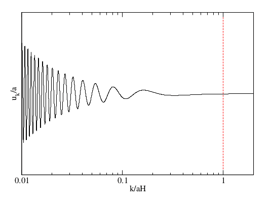
Fig 6. Evolution of a quantum fluctuation mode, $\delta \phi_k$, from its birth in the quantum vacuum out to superhorizon scales.

Note how the mode “freezes”, becoming constant as the wavelength grows to superhorizon scales. We are witnessing something quite profound here: we understand that the wavelike nature of the fluctuation on small scales is because it is fundamentally a quantum field. What are we to make of the smooth transition to a constant value on large scales? The quantum fluctuation has become a classical object upon attaining such dizzying growth: the wavefunction undergoes decoherence once it surpasses the causal limit of spacetime. Now a classical perturbation, the once nascent field fluctuation can influence the structure of spacetime, and, after the universe reheats, it will source acoustic disturbances in the baryon-photon plasma.

We are now finally ready to answer the question that launched this quest: what is the term $\langle | \delta \phi_k|^2\rangle$ appearing in Eq. (\ref{var})? First, we need to select a scale at which to evaluate it, seeing as it is a rapidly oscillating function of time. Since the fluctuation doesn’t become a bonified perturbation until it decoheres to a classical object on superhorizon scales, this is where we should evaluate $\delta \phi_k$. This important event—when the fluctuation transitions to superhorizon scales—is called horizon crossing and is marked by the condition $k=aH$. We’ll continue with our de Sitter space approximation so that we can more easily obtain a closed-form expression for $\langle | \delta \phi_k | \rangle^2$, but we’ll afterward discuss how we expect it to change when we let the dynamics become more general. What we want, then, is to evaluate Eq. (\ref{var}) at horizon crossing for each comoving scale, $k$,
$$
\langle | \delta_k|^2\rangle = \left. \left(\frac{H}{\dot{\phi}}\right)^2\langle | \delta \phi_k|^2\rangle \right|_{k = aH}.
$$
Now, rather than leave $\delta \phi_k$ in terms of Hankel functions, which are not especially user-friendly, we can simplify things considerably if we remember that $\delta \phi_k$ becomes constant on superhorizon scales. We can make this fact explicit in our expression by evaluating Eq. (\ref{ltmode}) in the long wavelength limit: $-k\tau \rightarrow 0$. Granted: $-k\tau \rightarrow 0$ is not the same as $-k\tau = k/aH = 1$, but since the mode settles down to a constant after horizon crossing this difference is immaterial. The asymptotic expressions of Bessel functions for small arguments are well-documented: in the limit $-k\tau \rightarrow 0$, the function $H^{(1)}_{3/2}(-k\tau)$ becomes $\sqrt{2/\pi}(k\tau)^{-3/2}$ and we get
$$
|\delta \phi_k| = \frac{|u_k|}{a} = \frac{H}{\sqrt{2k^3}},
$$
which leads to a final expression for the variance
\begin{equation}
\label{finalvar}
\langle | \delta_k|^2\rangle = \frac{H^4}{2\dot{\phi}^2 k^3}.
\end{equation}
This is an important result, but not the one I’d like to end with. Why do we care about the variance in the first place? Because it’s the Fourier transform of the spatial correlation function,
$$
\xi({\bf r}) = \langle \delta ({\bf x})\delta({\bf x} + {\bf r})\rangle = \frac{1}{(2\pi)^2}\int \langle| \delta_k|^2\rangle e^{-i{\bf k}\cdot{\bf r}}\,{\rm d}^3k.
$$
The function $\xi({\bf r})$ gives a measure of the lumpiness of the 3-dimensional density field throughout space and is especially interesting because it is due solely to quantum mechanical fluctuations—the seeds of density inhomogeneities that source the acoustic oscillations that we studied in the last section. As the embodiment of the correlation function in the frequency domain, the quantity $\langle | \delta_k|^2\rangle$ is called the power spectrum, though in the modern cosmology literature, the quantity is taken to be dimensionless,
\begin{equation}
\label{finalP}
P(k) = \frac{k^3}{2\pi^2} \langle | \delta_k|^2\rangle = \frac{1}{4\pi}\left.\frac{H^4}{\dot{\phi}^2}\right|_{k=aH},
\end{equation}
where we remind the reader that this quantity is the variance at horizon crossing, $k=aH$. This is the key result of this section, the so-called scalar power spectrum because it provides the initial conditions for density (scalar) perturbations in the post-inflationary era.

I mentioned earlier that, though we’d be developing this result, namely Eq. (\ref{finalP}), for the special case of de Sitter expansion, we would discuss how to modify it in the presence of more general cosmological dynamics. Indeed, as is, Eq. (\ref{finalP}) doesn’t even work in the de Sitter limit $H = const.$, because if $H$ is constant then $\dot{\phi} = 0$, and the fluctuation amplitude diverges badly⁶. How embarrassing. But, hold on. It turns out that, while this expression might have problems, we can use it as long as we stay away from pure de Sitter expansion. It works infinitesimally close to de Sitter. Since pure de Sitter expansion is defined as $H = {\rm const}$, we can model tiny deviations from de Sitter expansion by considering the lowest-order term in a Taylor expansion of the Hubble parameter,
$$
H(t) = H(t_0) + \dot{H}(t-t_0) + \cdots
$$
where we assume $\dot{H}/H^2$ is nonzero but still very much smaller than 1. Working in this limit of ever-so-close-to-de Sitter expansion, we can use this new expression to analytically study the scale dependence of the variance. Doing so will add some rigor to the rather heuristic discussion we gave in the context of Eq. (\ref{var}).

Recall that fluctuations on different length scales are sensitive to different periods throughout inflationary expansion: fluctuations on the largest length scales were nucleated earliest, and so were shaped by early-time inflationary dynamics, whereas smaller-scale fluctuations were affected by late-time dynamics. And, because fluctuations freeze when they surpass the horizon scale, they effectively “lock in” the dynamics up until this point of horizon crossing. We, therefore, make the following simple observation: the power spectrum on a scale $k$ is determined by the cosmological dynamics at the time when the scale coincides with the horizon, $k =aH$. The $k$-dependence of $P(k)$, only implicit in Eq. (\ref{finalP}), is encoded in the time-dependence of the cosmological parameters, $H$ and $\dot{\phi}$. We can establish a correspondence between time-scales and length-scales by differentiating $k=aH$ concerning time,
$$
\frac{{\rm d}k}{{\rm d}t} = \dot{a}H + a\dot{H} = kH\left(1+\frac{\dot{H}}{H^2}\right) \approx kH,
$$
from which we can write,
$$
{\rm d}\ln k = H {\rm d}t.
$$
In arriving here, we’ve discarded the term $\dot{H}/H^2$ because it’s so small. But wait—isn’t this the term we wish to keep to include deviations from pure de Sitter? Indeed, it is; however, this term is in the differential and, as it turns out, contributes at second-order to the power spectrum (e.g. leads to terms proportional to $\dot{H}^2/H^4$ which are super, super small). Now, let’s take the logarithm of Eq. \ref{finalP} and differentiate with respect to $\ln k$,
\begin{eqnarray}
\frac{{\rm d}\ln P(k)}{{\rm d} \ln k} &\propto & \frac{1}{H}\frac{{\rm d}}{{\rm d}t} \left(\ln H + \frac{1}{2}\ln \dot{\phi}\right) \\
&=& \frac{\dot{H}}{H^2} – \frac{\ddot{\phi}}{2H\dot{\phi}}.
\end{eqnarray}
Next, let’s write out the Taylor expansion of $\ln P(k)$,
\begin{eqnarray}
\label{TaylorP}
\ln \left(\frac{P(k)}{P(k_0)}\right) &=& \frac{{\rm d}\ln P(k)}{{\rm d}\ln k} \ln \left(\frac{k}{k_0}\right) + \cdots \nonumber \\
&=& (n(k_0) – 1)\ln \left(\frac{k}{k_0}\right) + \cdots
\end{eqnarray}
Writing this without the logarithms yields the well-known power law form of the power spectrum,
\begin{equation}
\label{PL}
P(k) = P(k_0) \left(\frac{k}{k_0}\right)^{n-1}.
\end{equation}
Here, $k_0$ is a reference wave number, known as the pivot scale. The number in the exponent, $n$, is the spectral index: comparison with Eq. (19) reveals that
\begin{equation}
n -1 = \left(\frac{\dot{H}}{H^2} – \frac{\ddot{\phi}}{2H\dot{\phi}}\right).
\end{equation}
Observe that, as we approach the de Sitter limit, $n \rightarrow 1$, and the spectrum approaches scale invariance. Any departure from scale invariance is proportional to the extent to which the background spacetime deviates from pure de Sitter. For approximately de Sitter expansion, we expect a power-law spectrum with a spectral index either slightly larger or smaller than unity: if $n < 1$, the spectrum is red, i.e. has more power (greater variance) on large length scales (to the “left” of the pivot); if $n > 1$, the spectrum is blue, i.e. has more power on small length scales (to the “right” of the pivot). Equation (\ref{PL}) is the analytical embodiment of the rather rough conceptual sketch behind Figures 30 and 31. In particular, the role of $\dot{\phi}$ in controlling the scale of the variance is taken up by the spectral index. Lastly, note the “$\cdots$” in the above expressions: we are free to consider higher-order modifications of the power spectrum, which will show up as $k$-dependent terms in the exponent of Eq. (\ref{PL}). In approximately de Sitter inflation, since higher-order time derivatives of $H$ and $\dot{\phi}$ are small, we likewise expect any departure from a power-law spectrum to be negligible.

In closing, we have shown how the quantum nature of the inflation field results in the generation of real, physical density perturbations in the baryon-photon plasma after inflation. These perturbations exist across a wide range of cosmological scales, and an important statistic tied to the inflationary dynamics is the variance of fluctuations as a function of scale. This statistic is provided by the power spectrum, $P(k)$, which takes the form of a power-law when the inflationary dynamics are close to de Sitter.

In writing this section to appeal to the poor man without significant knowledge of general relativity, quantum field theory, or cosmological perturbation theory, I have deviated somewhat from the standard treatment of inflationary fluctuations seen in the modern literature. In particular, Eq. (\ref{var}) is derived in a somewhat disjointed way, with the classical portion emerging readily from Eq. (\ref{dt}), but with the quantum fluctuation term requiring a rather more detailed excursion into the realm of quantum field theory in curved spacetime. The standard derivation of the density perturbation makes no such separation into classical and quantum parts, and furnishes the final result for the variance, Eq. (\ref{finalvar}), through a similar but more complete treatment⁷ of inflation fluctuations evolving in the inflationary universe. In presenting a less-advanced treatment of this subject, what we’ve sacrificed in terms of rigor I hope we’ve made up for in greater conceptual clarity: in particular, the role of the classical dynamics of inflation in modulating the variance of the quantum fluctuations is explicit in this presentation but quite obscure in the standard derivation. Those readers interested in tackling the complete theory are encouraged to consult the following reviews: [2-4]

References and Footnotes

[1] Abramowitz, M., Stegun, I. A., Handbook of Mathematical Functions with Formulas, Graphs, and Mathematical Tables, Dover (1960).
[2] Liddle, A. R., Lyth, D. H., The Cold dark matter density perturbation. Phys. Rept. 231, 1 (1993).
[3] Mukhanov, V. F., Feldman, H. A., Brandenberger, R. H., Theory of cosmological perturbations. Part 1. Classical perturbations. Part 2. Quantum theory of perturbations. Part 3. Extensions. Phys. Rept. 215, 203 (1992).
[4] Kodama, H., Sasaki, M., Cosmological Perturbation Theory. Prog. Theor. Phys. Suppl. 78, 1 (1984).

¹While $H$ varies during inflation, it’s typically very nearly constant in most models of interest, and so we assume $H$ does not change over the time it takes the separate regions within our Hubble sphere to stop inflating. back
²Scales of interest are length scales probable with cosmological data, like CMB and large-scale structure surveys. back
³Really what we’re considering here is the mode function associated with the positive frequency component of the quantized inflation vacuum fluctuation, i.e. the mode annihilated by the $\hat{a}_{\bf k}$ in the Fourier decomposition $\delta \phi = \int \frac{{\rm d}^3k}{(2\pi)^{3/2}}\left(\delta \phi_k(t)\hat{a}_{\bf k}e^{i{\bf k}\cdot{\bf r}}+\delta \phi_k^*(t)\hat{a}^\dagger_{\bf k}e^{-i{\bf k}\cdot{\bf r}}\right)$. back
⁴Note that these expressions differ from the case of a homogeneous scalar field. Because the field perturbations are functions of space, $\delta \phi ({\bf x},t)$, so too is the full field value, $\phi({\bf x},t) = \phi_0(t) + \delta \phi({\bf x},t)$. back
⁵Yes, the field fluctuation itself is being treated as a free quantum field here. back
⁶This divergence is actually a gauge artifact, but it does signal that we’re trying to do something nonphysical. It turns out that there actually aren’t any density perturbations in de Sitter inflation, for the simple fact that inflation never ends, anywhere. (Recall the critical role of $\delta t$—the time lag between reheating events across the universe—in the formation of density perturbations.) back
⁷The missing ingredient is the fact that the inflation fluctuations influence the background spacetime, creating curvature perturbations that in turn influence the evolution of the inflation. A complete treatment must include both curvature and inflation fluctuations in the equations of motion. back