Relativity Variables: Velocity, Doppler-Bondi k, and Rapidity

Traditional presentations of special relativity place emphasis on “velocity”, which of course has an important physical interpretation… carried over from Galilean physics. However, in many situations, working only with velocities can be tedious in calculations and may obscure the underlying geometry.

---

First, a story (inspired by my post in the recent Relativistic Relative Velocity thread). [Equations will be derived later.]
During my research meeting with my student (an undergraduate physics major), I posed the following question for him to work on [while I searched my computer for a file to print out for him]:

Given two identical particles with relative-velocity $\beta_{rel}=0.5$,
determine the relative velocity of the center-of-momentum frame.
[It’s not 0.25.]

• Velocity $\beta$ solution:He used the standard relative-velocity formula (velocity composition formula),
  $\beta_{rel}=\displaystyle\frac{\beta_2-\beta_1}{1-\beta_2\beta_1},$ with $\beta_2=-\beta_1$ (call it $\beta$), we have $\displaystyle \beta_{rel}=\frac{2\beta}{1+\beta^2}.$With $\beta_{rel}=0.5$, he solves the quadratic equation $\beta^2-4\beta+1=0$, with roots $2\pm\sqrt{3}$.
  (We discard the unphysical root $2+\sqrt{3}\approx 3.732$.)
  The physics answer is $\beta=2-\sqrt{3}\approx .268$.
• Doppler-Bondi $k$ solution:While he was completing his solution, I had found my file and tried to race him using another method: the [Doppler-]Bondi k-calculus, where $k=\displaystyle\sqrt{\frac{1+\beta}{1-\beta}}$ is the Doppler factor. The inverse relation is $\beta=\displaystyle\frac{k^2-1}{k^2+1}$. [Note: if we use the opposite velocity, the factor becomes its reciprocal. That is, when $\beta_{new}=-\beta_{old}$, then $k_{new}=k^{-1}_{old}$.]Relative-velocity is encoded by the relative-DopplerFactor formula:
  $k_{rel}=\displaystyle\frac{k_2}{k_1}$. [Multiplicatively, $k_2=k_{rel}k_1$.]
  For this problem, we have $k_{rel}=\displaystyle\frac{k}{k^{-1}}=k^2$. So, $k=\sqrt{k_{rel}}$.With $\beta_{rel}=0.5$, we have $k_{rel}=\sqrt{3}$. So, $k=\sqrt[4]{3}$.
  Thus, $\beta=\displaystyle\frac{\sqrt{3}-1}{\sqrt{3}+1}=2-\sqrt{3}\approx .268$.I would argue that this calculation is more efficient [assuming you know the relationships between $k$ and $\beta$ and the relative-DopplerFactor-formula]. These are the relationships used in my “Relativity on Rotated Graph Paper” Insight.

Is there a more efficient way?

• Rapidity $\theta$ solution:With rapidity $\theta$ (the Minkowski-spacetime analogue of the angle: the Minkowski-arc-length along the unit hyperbola or the area of its sector), where $\beta=\tanh(\theta)$ and $k=\exp(\theta)$,
  relative-velocity is encoded by the relative-rapidity formula:
  $\theta_{rel}=\theta_2-\theta_1$. [Additively, $\theta_2=\theta_{rel}+\theta_1$.]
  Geometrically, the center-of-momentum frame corresponds to the angle bisector of the worldlines of these equal-mass particles. So, the answer is immediately $\beta=\tanh\left(\frac{\rm arctanh(\beta_{rel})}{2}\right)$.
  With $\beta_{rel}=0.5$, we have $\beta=\tanh\left(\frac{\rm arctanh(0.5)}{2}\right)\approx 0.268$. (WolframAlpha gives 0.268.)
• Comments:
  • Since $\beta=0.5$ isn’t associated with a Pythagorean triple (or equivalently, a rational Doppler factor), the numbers are ugly and require a calculator. Please use $3/5$ or $4/5$ or $5/13$, etc… if you can.
  • Given the way that introductory textbooks are currently written, Bondi-k and rapidity methods may be too advanced for introductory students… but the mathematics is probably not really much more complicated than the trigonometry in a free-body diagram.
    These approaches are more appropriate for intermediate undergraduate majors.
  • Clearly, the rapidity [angle] solution reveals the geometrical situation best.

---

relationships among Velocity $\beta$, Doppler-Bondi $k$, and Rapidity $\theta$

We now proceed to show the relationships among these parameters–to help facilitate moving from one representation to another.

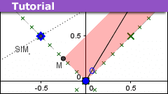
Here is a GeoGebra visualization to show the relationships.

https://www.geogebra.org/m/bFxv6tja

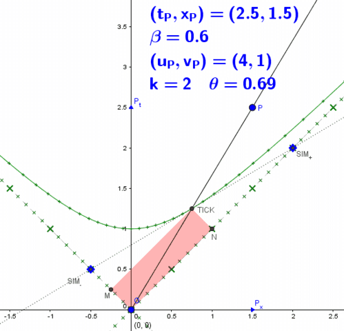
Time runs upwards. Rapidity is the Minkowski-arc-length along the unit hyperbola. The lightcone coordinates $(u,v)$  have $u$ along the future-forward lightcone and $v$ along the future-backward lightcone. The Doppler-Bondi $k$-factor is the eigenvalue along the future-forward direction, which stretches the light-clock diamond in that direction by a factor $k$. The reciprocal $k^{-1}$ is the eigenvalue along the future-backward direction, which shrinks the light-clock diamond by a factor of $k$. Note the light-clock diamond area is preserved. This is the basis of my “Relativity on Rotated Graph Paper” Insight.

 

---

Now, we develop the formulas (hopefully with all the correct signs)…

• velocity $v$The Lorentz Transformation in velocity-form:
  $\begin{pmatrix} t_P’\\ x_P’ \end{pmatrix} = \begin{pmatrix} \frac{1}{\sqrt{1-\beta^2}}&\frac{-\beta}{\sqrt{1-\beta^2}}\\ \frac{-\beta}{\sqrt{1-\beta^2}}&\frac{1}{\sqrt{1-\beta^2}}\\ \end{pmatrix} \begin{pmatrix} t_P\\ x_P \end{pmatrix} = \begin{pmatrix} \gamma&-\beta\gamma\\ -\beta\gamma&\gamma\\ \end{pmatrix} \begin{pmatrix} t_P\\ x_P \end{pmatrix}$, where $\gamma\equiv\displaystyle\frac{1}{\sqrt{1-\beta^2}}$.(Note the Euclidean analogue of this is a “rotation in slope-form”:
  $\begin{pmatrix} t_P’\\ x_P’ \end{pmatrix} = \begin{pmatrix} \frac{1}{\sqrt{1+m^2}}&\frac{-m}{\sqrt{1+m^2}}\\ \frac{m}{\sqrt{1+m^2}}&\frac{1}{\sqrt{1+m^2}}\\ \end{pmatrix} \begin{pmatrix} t_P\\ x_P \end{pmatrix}$.)The determinant of the Lorentz Transformation is $\gamma^2-(-\beta\gamma)^2=\gamma^2(1-\beta^2)=1$.
  The trace is $\gamma+\gamma=2\gamma$.
  By composing two transformations, we obtain another Lorentz transformation
  $\begin{eqnarray*} \begin{pmatrix} \gamma_{2}&-\beta_{2}\gamma_{2}\\ -\beta_{2}\gamma_{2}&\gamma_{2}\\ \end{pmatrix} &= \begin{pmatrix} \gamma_{rel}&-\beta_{rel}\gamma_{rel}\\ -\beta_{rel}\gamma_{rel}&\gamma_{rel}\\ \end{pmatrix} \begin{pmatrix} \gamma_{1}&-\beta_{1}\gamma_{1}\\ -\beta_{1}\gamma_{1}&\gamma_{1}\\ \end{pmatrix}\\ &= \begin{pmatrix} \gamma_{rel}\gamma_{1}(1+\beta_{rel}\beta_1)&-\gamma_{rel}\gamma_{1}(\beta_{rel}+\beta_1)\\ -\gamma_{rel}\gamma_{1}(\beta_{rel}+\beta_1)& \gamma_{rel}\gamma_{1}(1+\beta_{rel}\beta_1)\\ \end{pmatrix} \end{eqnarray*}$By factoring,
  $\begin{eqnarray*} \gamma_2\begin{pmatrix} 1&-\beta_{2}\\ -\beta_{2}&1\\ \end{pmatrix} &= \gamma_{rel}\gamma_{1}(1+\beta_{rel}\beta_1)\begin{pmatrix} 1&-\frac{(\beta_{rel}+\beta_1)}{(1+\beta_{rel}\beta_1)}\\ -\frac{(\beta_{rel}+\beta_1)}{(1+\beta_{rel}\beta_1)}&1\\ \end{pmatrix} \end{eqnarray*}$,
  we see the velocity-composition formula: $\beta_2=\displaystyle\frac{\beta_{rel}+\beta_1}{1+\beta_{rel}\beta_1}$.

---

introducing Doppler-Bondi $k$ and the Rapidity $\theta$

Let’s find the eigenvalues [call them $k$’s] and eigenvectors of the Lorentz Transformation.
What vectors $\vec w$ satisfy $M\vec w=k\vec w$ for some $k$?

Before we get into the details of a brute-force calculation, let’s deduce some properties.
Call $k_{+}$ and $k_{-}$, the larger and smaller of the two eigenvalues.
When we are done, we expect the Lorentz Transformation, expressed in the eigenbasis [to be determined] to take the form
$\begin{pmatrix} k_{+}&0\\ 0&k_{-}\\ \end{pmatrix}.$
Since the determinant will still be $1$, we deduce that $k_{-}=1/k_{+}$.
So, let’s call $k_{+}$ simply $k$, and thus $k_{-}$ is $k^{-1}$.
Thus, we have
$\begin{pmatrix} k&0\\ 0&k^{-1}\\ \end{pmatrix}.$

By composition, we have
$\begin{pmatrix} k_2&0\\ 0&k_2^{-1}\\ \end{pmatrix}=\begin{pmatrix} k_{rel}&0\\ 0&k_{rel}^{-1}\\ \end{pmatrix} \begin{pmatrix} k_1&0\\ 0&k_1^{-1}\\ \end{pmatrix}$, so that $k_2=k_{rel}k_1$, or $k_{rel}=\displaystyle\frac{k_{2}}{k_{1}}$.

Possibly by a leap of faith, this multiplicative relation can be expressed in terms of an additive parameter [call it $\theta$]: write $k=\exp\theta$ so that $k_2=k_{rel}k_1$ can be written as $\exp(\theta_2)=\exp(\theta_{rel})\exp(\theta_1)$. This means that $\theta_2=\theta_{rel}+\theta_1$, or equivalently $\theta_{rel}=\theta_2-\theta_1$.

 

Since the trace will still be $2\gamma$, we deduce that $\gamma=\displaystyle\frac{k_{+}+k_{-}}{2}=\frac{k+k^{-1}}{2}$.
To solve for $k$, we obtain a quadratic equation: $0=k^2-2\gamma k+1$ that is solved by $k_{\pm}=\gamma\pm\sqrt{\gamma^2-1}=\gamma\pm\gamma\sqrt{1-\gamma^{-2}}=\gamma\pm\gamma\sqrt{1-(1-\beta^2)}=\gamma\pm\gamma\beta=\gamma(1\pm\beta)=\sqrt{\frac{1\pm \beta}{1\mp\beta}}$.

This is the Doppler formula (although, at this point, it may not be clear what this means).

Using $k=\exp\theta$, we see that $\gamma=\displaystyle\frac{k+k^{-1}}{2}=\frac{\exp(\theta)+\exp(-\theta)}{2}=\cosh\theta$.

Since [from the determinant relation] $\gamma^2-(\beta\gamma)^2=1$, we find $(\beta\gamma)^2=\gamma^2-1=\cosh^2\theta-1=\sinh^2\theta$ and thus $\beta\gamma=\sinh\theta$ and $\beta=\frac{\sinh\theta}{\gamma}=\frac{\sinh\theta}{\cosh\theta}=\tanh\theta$.

We’ll summarize the equations at the end.

 

---

Okay back to the eigenvector problem.

Solve the characteristic equation for $k$: $0=\det (M-kI)=\det\begin{pmatrix} \gamma-k&-\beta\gamma\\ -\beta\gamma&\gamma-k\\ \end{pmatrix}=(\gamma-k)^2-(-\beta\gamma)^2$.
[If you expand this out, you’ll find that this yields the quadratic equation for $k$ ($0=k^2-2\gamma k+1$) we obtained earlier using the trace and the determinant.]
So, $k-\gamma=\pm\beta\gamma$, or
$k=\gamma(1\pm\beta)=\frac{(1\pm\beta)}{\sqrt{1-\beta^2}}=\sqrt{\frac{(1\pm\beta)^2}{(1-\beta)(1+\beta)}}=\sqrt{\frac{1\pm\beta}{1\mp\beta}}$, which are the Doppler factors [as now expected].

 

The eigenvector corresponding to $k=k_{+}=\gamma(1+\beta)$ is gotten by substitution:

$\begin{pmatrix} 0 \\ 0\end{pmatrix}= \begin{pmatrix} \gamma-(\gamma(1+\beta))&-\beta\gamma\\ -\beta\gamma&\gamma-(\gamma(1+\beta))\\ \end{pmatrix}\begin{pmatrix} w_t \\ w_x\end{pmatrix}=\begin{pmatrix} -\beta\gamma & -\beta\gamma  \\-\beta\gamma  & -\beta\gamma \end{pmatrix}\begin{pmatrix} w_t \\ w_x\end{pmatrix}=\begin{pmatrix} (-\beta\gamma)w_t +  (-\beta\gamma)w_x \\ (-\beta\gamma)w_t +  (-\beta\gamma)w_x\end{pmatrix}$.

This is satisfied by vectors of the form $w_x=w_t$–that is, the along the future-forward lightlike direction. Thus, under a Lorentz Transformation, the light-signal’s velocity remains unchanged, but the future-forward component of a vector gets stretched by a factor of $k$. Similarly, the future-backward component gets reduced by a factor of $k$. This is the area-preserving transformation of the causal diamonds from my “Relativity on Rotated Graph Paper” Insight.

---

SUMMARY of Equations

So, we have

$k=e^\theta=\cosh\theta+\sinh\theta=\cosh\theta(1+\tanh\theta)=\gamma(1+\beta)$

$1/k=e^{-\theta}=\cosh\theta-\sinh\theta=\cosh\theta(1-\tanh\theta)=\gamma(1-\beta)$

By multiplication, $1=\gamma^2(1-\beta^2)$.

By division, $k^2=e^{2\theta}=\frac{1+\beta}{1-\beta}$.

Half-the-difference is $\frac{1}{2}(k-k^{-1})=\sinh\theta=\cosh\theta \tanh\theta=\gamma \beta$.

Half-the-sum is $\frac{1}{2}(k+k^{-1})=\cosh\theta=\gamma$.

The ratio is $\beta=\tanh\theta=\frac{k-k^{-1}}{k+k^{-1}}=\frac{k^2-1}{k^2+1}$.

• applications to Velocity composition$\theta_{rel}=\theta_2-\theta_1$
  implies, by exponentiation,
  $\exp\theta_{rel}=\exp\theta_2-\exp\theta_1$, or  $k_{rel}=\displaystyle\frac{k_2}{k_1}$Using $\beta=\tanh\theta$,
  we have
  $\begin{align*} \beta_{rel} &=\tanh\theta_{rel}\\ &=\tanh(\theta_2-\theta_1)\\ &=\displaystyle\frac{\tanh\theta_2-\tanh\theta_1}{1-\tanh\theta_2\tanh\theta_1}\\ &=\displaystyle\frac{\beta_2-\beta_1}{1-\beta_2\beta_1} \end{align*}$
• application to the Lorentz transformations$\begin{pmatrix} \gamma&-\beta\gamma\\ -\beta\gamma&\gamma\\ \end{pmatrix} =\begin{pmatrix} \cosh\theta&-\sinh\theta\\ -\sinh\theta&\cosh\theta\\ \end{pmatrix} =\cosh\theta\begin{pmatrix} 1 &-\tanh\theta\\ -\tanh\theta&\ 1\\ \end{pmatrix}$Note: from the composition of transformations,
  $\begin{align*} \gamma_2 &=\gamma_{rel}\gamma_{1}(1+\beta_{rel}\beta_1)\\ &=\cosh\theta_{rel}\cosh\theta_1(1+\tanh\theta_{rel}\tanh\theta_1)\\ &=\cosh\theta_{rel}\cosh\theta_1+\sinh\theta_{rel}\sinh\theta_1)\\ &=\cosh(\theta_{rel}+\theta_1)\\ &=\cosh( (\theta_2-\theta_1) + \theta_1)\\ &=\cosh( \theta_2)\\ \end{align*}$

There’s more to the story… but this will have to do until then.

---

It seems “rapidity” was defined by A.A. Robb in his 1911 “Optical Geometry of Motion“.

Hermann Bondi‘s k-calculus is developed in his 1962 “Relativity and Common Sense“.
Aspects of the method appeared in Robb’s book and in Milne’s 1935 “Relativity, Gravitation and World-Structure“.