Explore Coordinate Dependent Statements in an Expanding Universe

In this Insight, we will discuss the general Robertson-Walker (RW) universe, in which a set of co-moving observers with proper time $t$ observe the universe to be homogeneous and isotropic. In such a universe, the line element takes the form
$$ds^2 = dt^2 – a(t)^2 [dr^2 + f(r)^2 d\Omega^2] \equiv dt^2 – a(t)^2 dS^2,$$
where $f(r) = r$ in the case of a spatially flat universe, $f(r) = R \sin(r/R)$ for a closed universe, and $f(r) = R \sinh(r/R)$ for an open universe. For the sake of the argument, we will restrict ourselves to the case of one spatial dimension, but the ideas readily generalize to three spatial dimensions.

Although the actual computations are generally not difficult, the Insight is written at intermediate to advanced level and assumes that the reader is already familiar with basic concepts in general relativity as well as cosmology. We will also not deal with the energy content of the universe and how it relates to the time evolution of the scale factor $a(t)$, but instead focus on the local relation between comoving observers and the relation between Doppler shift and cosmological redshift. In particular, we will demonstrate how any splitting into Doppler shift and cosmological redshift is artificial and a result of the choice of coordinates.

Throughout this Insight, we will use units in which $c = 1$ and the metric signature $+ – – -$.

Comoving Coordinates and the Expansion of the Universe

Within the area of cosmology, comoving coordinates is so convenient and used so frequently that many interpretations of physical results that you will find in textbooks do not even bother to point out which descriptions are coordinate independent and which are interpretations based on the choice of coordinates. Let us briefly go through some of those coordinate-dependent concepts:

• Age of the universe: Considering a universe that is born at time $t = 0$, the coordinate $t = t_0$ today is considered to be the age of the universe. It is what is generally referred to when cosmologists tell you that the universe is almost 14 billion years old. In reality, this is the time passed for a comoving observer at constant $x$, since $ds = dt$ for such observers. Since the world lines of comoving observers are geodesics, this is the maximal possible time any observer can experience between $t = 0$ and $t = t_0$.
• The universe at a given time: As we learned in special relativity, what constitutes a moment in time is observer-dependent or, more precisely, dependent on the simultaneity convention. In special relativity, the common thing to do is to consider Minkowski coordinates and different simultaneity conventions follow from different inertial frames. However, we can a priori adopt any simultaneity convention that foliates space-time into a set of space-like hypersurfaces where we can talk about each hypersurface as “the universe at a specific moment in time”. In practice, the usual thing to do in cosmology is to talk about a foliation using the hypersurfaces of fixed $t$ coordinate. However, we could in principle also imagine other foliations. In particular, we could look at a local region of space-time small enough for curvature effects to be negligible and consider a local Minkowski frame with its corresponding (local) simultaneity convention. As we shall see, this simultaneity convention is generally not the same as that using the hypersurfaces of fixed cosmological time $t$.
• Proper distance: As we also learned in special relativity, distance is not invariant. A crucial part of the derivation of length contraction is to figure out which events we should be comparing to know the length of an object and the answer to this question is events at the ends of the object that are simultaneous. In cosmology, it is common to refer to the proper distance between two objects as the distance between them at a given time (see above!). This distance should be computed using the induced metric on the hypersurface of simultaneity, which will be a Riemannian metric since it is a space-like surface. In the case of the RW universe, this metric is given by the line element $d\Sigma^2 = a(t)^2 dS^2$, where the $t$ depends on which moment in time we are looking at. It is also common to talk about the comoving distance between two objects, which is just the proper distance divided by the scale factor $a(t)$. For two comoving observers, the comoving distance is constant while the proper distance increases linearly with the scale factor.

So what do we mean when we say that an RW universe is expanding? It just means that the proper distance between comoving observers increases with time. (Note how we threw in the definition of simultaneity as well as proper distance here, both discussed above!) Due to the comoving distance between comoving observers being constant, mathematically this just means that $a'(t) > 0$.

Christoffel symbols of the comoving coordinates

It is a worthwhile exercise in itself to compute the Christoffel symbols in comoving coordinates. For the sake of the argument, we will here only do so explicitly for a $1+1$-dimensional RW universe for which
$$ds^2 = dt^2 – a(t)^2 dx^2,$$
since this will be sufficient for our purposes. From now on, we will not write out the time dependence of the scale factor $a$. Instead, this will be implicit everywhere.

Given the line element for our $1+1$-dimensional RW universe, the geodesic equations will be given by finding the extrema of the functional
$$\mathcal S = \int \mathcal L \, d\tau, \quad \mbox{where} \quad \mathcal L = \dot t^2 – a^2 \dot x^2$$
and the dot represents differentiation concerning the proper time $\tau$. The Euler–Lagrange equations now directly lead to
$$\ddot t + a a’ \dot x^2 = 0 \quad \mbox{and} \quad 0 = \frac{d}{d\tau} a^2 \dot x = a^2 \ddot x + 2 a a’ \dot x \dot t.$$
The non-zero Christoffel symbols of this space-time can be directly read as
$$\Gamma^t_{xx} = aa’ \quad \mbox{and} \quad \Gamma^x_{xt} = \Gamma^x_{tx} = \frac{a’}{a}.$$
The exact form of these Christoffel symbols is not as relevant to our upcoming discussion as the fact that they are generally non-zero whenever $a’ \neq 0$. In particular, this is the case in an expanding universe.

The Local Minkowski Frame

A basic result in differential geometry is that regardless of what the metric tensor is, it is always possible to find a coordinate system such that for some given point $p$ in the manifold, not only is the coordinate basis orthonormal but additionally all first-order partial derivatives of the metric components vanish. We will call such a coordinate system a local Minkowski frame. In particular, this implies that all of the Christoffel symbols of the Levi-Civita connection are zero at $p$ as they can be written in terms of the metric components and their first-order partial derivatives. Hence, the comoving coordinate system does not have this property unless $a’ = 0$. We will here start by explicitly constructing a coordinate system that does have this property and then discussing its relation to the comoving coordinate system.

The construction of a local Minkowski frame can be made rather straightforward through exponentiation of the tangent space at $p$, leading to so-called normal coordinates. However, for our purposes, it is sufficient to look at the coordinate functions up to the second order in the coordinate differences from $p$. Letting $x^a$ be a general coordinate system with Christoffel symbols $\Gamma^a_{bc}$, we can assume that the coordinates $x^a = 0$ correspond to the point $p$ without loss of generality and set out to construct coordinates $\xi^\mu$ where the Christoffel symbols vanish. Additionally, we will require that $\xi^\mu$ is orthonormal at $p$, i.e., that $g(\partial_\mu,\partial_\nu) = \eta_{\mu\nu}$. We can do this by selecting any orthonormal vectors $e_\mu$ at $p$ and requiring that $\partial_\mu = e_\mu$, leading to
$$\partial_\mu = \frac{\partial x^a}{\partial \xi^\mu} \partial_a = e_\mu^a \partial_a \quad \Longrightarrow \quad \frac{\partial x^a}{\partial \xi^\mu} = e_\mu^a,$$
where $e_\mu^a$ are the components of $e_\mu$ in the $x^a$ coordinate system. Furthermore, the second derivatives of $x^a$ concerning $\xi^\mu$ can be found by requiring that the Christoffel symbols in the $\xi^\mu$ coordinate system vanish at $p$ and using the transformation rule of the Christoffel symbols
$$\Gamma^\mu_{\nu\sigma} = e^\mu_a e^b_\nu e^c_\sigma \Gamma^a_{bc} + e^\mu_a \frac{\partial^2 x^a}{\partial\xi^\nu \partial \xi^\sigma},$$
where $e^\mu$ are the dual vectors such that $e^\mu(e_\nu) = \delta^\mu_\nu$. However, this transformation rule is rather cumbersome to implement and we can instead use the fact that the vanishing of the Christoffel symbols should lead to the geodesic equations taking the form
$$\ddot \xi^\mu = 0$$
at $p$. In the $x^a$ coordinates, the geodesic equations are of the form
$$\ddot x^a + \Gamma^a_{bc} \dot x^b \dot x^c = 0$$
and expanding $x^a$ to second order in $\xi^\mu$ generally leads to
$$x^a = e^a_\mu \xi^\mu + c^a_{\mu\nu} \xi^\mu \xi^\nu + \mathcal O_3,$$
where we have introduced the notation $\mathcal O_n$ for terms that are of order three or higher in the coordinates. Inserting this into the geodesic equation and using that $\ddot \xi^\mu = 0$ results in
$$2 c^a_{\mu\nu} \dot\xi^\mu \dot\xi^\nu + e^b_\mu e^c_\nu \Gamma^a_{bc} \dot\xi^\mu \dot\xi^\nu + \mathcal O_1 = 0$$
from which we can identify
$$c^a_{\mu\nu} = – \frac{1}{2} e^b_\mu e^c_\nu \Gamma^a_{bc}$$
to leading order in $\xi^\mu$. The coordinate transformation from the local Minkowski frame to $x^a$ is therefore given by
$$x^a = e^a_\mu \xi^\mu – \frac{1}{2} e^b_\mu e^c_\nu \Gamma^a_{bc} \xi^\mu \xi^\nu + \mathcal O_3,$$
which can be easily inverted to
$$\xi^\mu = e_a^\mu x^a + \frac{1}{2} e_a^\mu \Gamma^a_{bc} x^b x^c + \mathcal O_3.$$

Comoving observers in a local Minkowski frame

Let us apply what we just learned to the $1+1$-dimensional space-time we discussed above. We will use $x$ and $t$ as our RW coordinates and $\xi$ and $\tau$ for our local Minkowski frame. Note that we will here use $t = 0$ at the point $p$, but there is nothing particular about this choice unless we do the usual cosmological assumption that $t = 0$ corresponds to the beginning of the universe. If you feel uncomfortable with this, replace every instance of $t$ below with $t-t_0$, where $t_0$ is the comoving time at which we want to construct the local Minkowski frame.

Since the non-zero components of the metric are $g_{tt} = 1$ and $g_{xx} = -a^2$, the RW coordinates are already orthogonal and we can choose $e_\tau = \partial_t$ and $e_\xi = a_0^{-1} \partial_x$, where $a_0 = a(0)$ is the scale factor at $p$. This directly leads to
\begin{align*}
t&\simeq
\tau – \frac{1}{2} \Gamma^t_{xx} e^x_\xi e^x_\xi \xi^2
= \tau -\frac{1}{2}H_0 \xi^2, \\
a_0 x &\simeq \xi – a_0 \Gamma^x_{tx} e^t_\tau e^x_\xi \tau \xi
= \xi(1 – H_0 \tau),
\end{align*}
where the $\simeq$ represents equality up to $\mathcal O_3$ and we have introduced the Hubble parameter $H_0 = a’_0/a_0$ at $p$. The inversion of this coordinate relation is given by
\begin{align*}
\tau &\simeq t + \frac{1}{2}H_0 a_0^2 x^2 = t + \frac{1}{2} a’^2_0 x^2, \\
\xi &\simeq a_0 x (1 + H_0 t).
\end{align*}

So what does the above tell us about our local Minkowski frame about the comoving frame? Considering the same type of local simultaneity convention as that found in special relativity we would conclude that it is surfaces of constant $\tau$, not constant $t$, that are simultaneity surfaces and the $\xi$ coordinate difference with this simultaneity convention that represent distances. Since all comoving observers have constant $x$, we find that a comoving observer at distance $\xi_0 = d_0$ from $\xi = 0$ at $\tau = 0$ has a world line that is given by
$$\xi \simeq d_0 (1 + H_0 \tau).$$
In other words, in the local Minkowski frame, this comoving observer is moving away from $\xi = 0$ with velocity $v = H_0 d_0$, which is just Hubble’s law. This underlines the main point. While comoving observers in RW coordinates are at rest and the distance between them grows due to expansion, the distances in the local Minkowski frame grow due to the comoving observers moving apart. Both descriptions are valid interpretations of observations, but each is based on a particular choice of coordinates and neither can be said to be more correct than the other.

Doppler Shift Versus Cosmological Redshift

Another thing that you may see in various sources is discussions about redshift as an effect of expansion, the so-called cosmological redshift. It is sometimes ascribed to the expansion “stretching” of the wavelength of the light signals, alternatively the distance between consecutive signals. After reading up to this point, your warning bells should all already be sounding loud, and recognize this as a coordinate-dependent statement. Indeed, in RW coordinates, the expansion of the universe does increase the distance between consecutive signals, but this does not a priori tell us that the same interpretation will explain the redshift in other coordinate systems. In particular, any attempt to ascribe part of any redshift to expansion and part to motion is doomed to be coordinate-dependent as we have already seen that simultaneity, distances, and velocities are coordinate-dependent.

In what follows, we will discuss the standard treatise of Doppler shift in special relativity and cosmological redshift in RW coordinates before discussing how they are two faces of the same coin. We will discuss what frequency means in general relativity and how this translates to the special cases of Doppler shift and cosmological redshift. This will allow us to come to a unified description of redshift in general and illustrate that ascribing it to expansion in the case of RW coordinates is a matter of coordinate convention.

Doppler shift

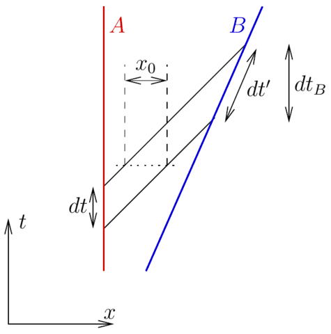
Figure 1. Two light signals sent from observer $A$ to observer $B$ with a proper time delay $dt$ for $A$, equal to the coordinate time difference in the rest frame of $A$. The time difference in the same frame between the observation of the signals by $B$, who is moving to the right at velocity $v$ is $dt_B$, which is time dilated relative to the proper time $dt’$ of $B$.

Consider two observers $A$ and $B$ such that $B$ travels away from $A$ with speed $v$ in the rest frame of $A$. At time $t = t_0$, $A$ sends a light signal towards $B$ followed by another signal a time $dt$ later, i.e., at $t = t_0 + dt$. This situation is shown in terms of a Minkowski diagram in Figure 1. For $A$, the time between the signals is $dt$. When the first pulse arrives at $B$, the second is a distance $x_0 = dt$ behind (remember, we are using units where $c = 1$). Since $B$ is moving away from $A$, the second signal will not reach $B$ until a time $dt_B$ later, where
$$x_0 + v\, dt_B = dt_B \quad \Longrightarrow \quad dt_B = \frac{dt}{1-v}.$$
This time difference is related to the proper time $dt’$ of $B$ between receiving the pulses according to the standard time dilation formula
$$dt’ = \frac{dt_B}{\gamma} = \frac{dt \sqrt{1-v^2}}{1-v} = dt \sqrt{\frac{1+v}{1-v}}.$$
If we let $dt$ and $dt’$ represent the times between consecutive wave crests in a light wave, the frequencies of the wave that $A$ and $B$ observe are proportional to the reciprocal of $dt$ and $dt’$, respectively, leading to
$$\frac{f_B}{f_A} = \frac{dt}{dt’} = \sqrt{\frac{1-v}{1+v}},$$
which is the standard Doppler shift formula for an observer moving away from the source.

Cosmological redshift

The standard treatment of cosmological redshift in RW coordinates is to similarly consider two observers $A$ and $B$, with the difference that they are now comoving. Without loss of generality we can consider $A$ to be at the comoving origin and $B$ to be located a comoving distance $x_0$ away, i.e., $x_A = 0$ and $x_B = x_0 > 0$. Again, we will consider the $1+1$-dimensional space-time from above, but nothing changes when looking at a higher-dimensional space-time. We assume that $A$ send the signal towards $B$ at cosmological time $t = t_1$ and that $B$ receives the signal at $t = t_2$. Furthermore, like above, $A$ sends a second signal at a proper time $d\tau$ after $t_1$ and $B$ receives the second signal a proper time $d\tau’$ after $t_2$. Note that, since both $A$ and $B$ are comoving, $d\tau$ and $d\tau’$ are just the corresponding differences in the cosmological time between the first and second signals.

Since the light signals follow a null geodesic, we can find their world lines rather easily. Since a null geodesic satisfies
$$ds^2 = dt^2 – a^2 dx^2 = 0,$$
it follows that
$$\frac{dt}{a} = \pm dx,$$
where the positive sign is for a signal moving in the positive direction, which is what we are considering here. Integrating this from $x = 0$ to $x = x_0$ for the first signal leads to
$$x_0 = \int_0^{x_0} dx = \int_{t_1}^{t_2} \frac{dt}{a}$$
while the corresponding integral for the second signal is given by
$$x_0 = \int_{t_1 + d\tau}^{t_2 + d\tau’} \frac{dt}{a}.$$
Since both expressions for the comoving distance must agree, it follows that
$$\int_{t_2}^{t_2+d\tau’} \frac{dt}{a} = \int_{t_1}^{t_1+d\tau} \frac{dt}{a}$$
and for small enough $d\tau$ this can be well approximated by
$$\frac{d\tau’}{a_2} = \frac{d\tau}{a_1} \quad \Longrightarrow \quad \frac{f_B}{f_A} = \frac{d\tau}{d\tau’} = \frac{a_1}{a_2},$$
where $a_i = a(t_i)$. The frequency observed by $B$ is therefore redshifted by the quotient of the scale factors at the time of emission and the time of detection, exactly corresponding to a stretch of the wavelength by $a_2/a_1$, since the speed of light is the same for either observer.

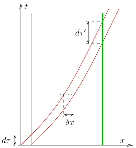
Figure 2. A representation of two consecutive light signals (red) sent from one comoving observer (blue) to the other (green) in comoving coordinates with a proper time difference $d\tau$ for the sending observer between the emissions. The comoving distance $\delta x$ between the signals remains the same, but the comoving speed $dx/dt$ decreases due to the expansion of the universe. This leads to the proper time $d\tau’$ between the signals for the receiving observer being larger.

Alternatively, this can also be seen graphically, see Figure 2. Assuming that the time $d\tau$ is small enough for the universe not to expand significantly between the emissions, we would find that the comoving distance between the signal at the time of the second emission is given by $\delta x = d\tau/a_1$. Due to the homogeneity of the universe, $x(t) + \delta x$ must be a null geodesic if $x(t)$ is a null geodesic and the signals, therefore, maintain their comoving separation throughout the propagation, meaning that the second signal will still be a comoving distance $\delta x$ behind when the first signal arrives at $B$. Since the proper distance corresponding to $\delta x$ is now $a_2 \delta x$, it takes another $d\tau’ = a_2 dt/a_1$ for the second signal to arrive. Seeing the signals as consecutive wave crests of a single light signal, has exactly the interpretation of stretching the wavelength through the expansion.

What is an observed frequency?

For every wave or periodic phenomenon, we can define a phase function $\phi$ in such a way that it increases by one for every wave crest or pulse. This is a scalar function on space-time and for a plane wave in Minkowski space, it is given by $\phi = k_\mu x^\mu/2\pi$, where $k$ is the wave 4-vector. For any observer, the frequency $f$ of the phenomenon is the derivative of $\phi$ concerning the observer’s proper time $\tau$ along the observer world line. Using the chain rule, this can be written on the form
$$\frac{d\phi}{d\tau} = \frac{\partial\phi}{\partial x^\mu} \frac{dx^\mu}{d\tau} = d\phi(V) \equiv N\cdot V,$$
where $d\phi$ is the exterior derivative of $\phi$ (i.e., a one-form) and $V$ is the observer’s 4-velocity. The 4-frequency $N$ is the tangent vector associated with $d\phi$ by the inverse metric tensor. This is illustrated for a plane wave in Minkowski space in Figure 3.

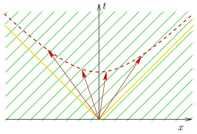
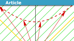
Figure 3. The level curves of the phase function $\phi$ corresponding to a plane wave moving to the right are shown in green. For an observer at the origin, the frequency of the wave can be inferred from the product of $d\phi$ and the observer 4-velocity, essentially the number of level curves the 4-velocity crosses. A set of possible observer 4-velocities is shown as red vectors. Any 4-velocity at the origin will end on the red dashed hyperbola. We can here see graphically that an observer traveling in the same direction as the wave will observe a lower frequency than an observer traveling in the opposite direction. The yellow lines represent the future light cone of the origin.

When we consider light signals or a train of light pulses, the phase function is constant along the future light cones of the signal source. Since any light cone is a null surface, $d\phi(N) = 0$ everywhere. As long as the connection is the Levi-Civita connection as is usually assumed, $d\phi$ is parallel transported along the null geodesics of the light cone as
$$\nabla_N \nabla_\mu \phi = g^{\nu\sigma} (\nabla_\nu \phi) (\nabla_\sigma \nabla_\mu \phi)
= \frac{1}{2} \nabla_\mu [g^{\nu\sigma} (\nabla_\sigma \phi) (\nabla_\nu\phi)]
= \frac{1}{2} \nabla_\mu 0 = 0,$$
where we have used that the connection is both metric compatible and torsion-free as well as that $d\phi$ is null. This means that we will be able to compute the observed frequency for any observer by parallel transporting the $d\phi$ of the emitted signal along the null geodesic from the source event to the receiver event, which also has $N$ as its tangent vector, and there take the inner product with the observer 4-velocity.

Note that, since inner products are preserved by parallel transport, we could just as well parallel transport the observer 4-velocity to the point of emission and there take the inner product with $d\phi$, which will lead to the same result but may or may not be an easier computation.

Application to the Doppler shift

In the case of the Doppler shift discussed above, assuming that $x_B > x_A$, the signals are sent in the positive $x$-direction and therefore the geodesic along which a signal travels has a tangent vector $N = f_0(\partial_t + \partial_x)$, where $f_0$ is some constant, leading to $d\phi = f_0(dt – dx)$. In the rest frame of the source $A$, its 4-velocity is $V_A = \partial_t$ and the frequency observed by the source is therefore
$$f_A = d\phi(V_A) = f_0 [dt(\partial_t) – dx(\partial_t)] = f_0.$$
Since Minkowski space is flat and all Christoffel symbols vanish in standard Minkowski coordinates, it does not matter which curve we parallel transport $d\phi$ along to get to the observer, it will always be given by $d\phi = f_0(dt – dx)$ at any point on the light cone. Since $B$ is moving away from $A$ with velocity $v$, its 4-velocity is given by $V_B = \gamma(\partial_t + v \partial_x)$ and the frequency observed by $B$ is therefore
$$f_B = d\phi(V_B) = f_0\gamma [dt(\partial_t + v\partial_x) – dx(\partial_t + v\partial_x)]
= f_0 \frac{1-v}{\sqrt{1-v^2}} = f_A \sqrt{\frac{1-v}{1+v}}.$$
This is the same Doppler shift formula as the one we found above.

Application to cosmological redshift

Going back to the description of cosmological redshift in RW coordinates, the signal emitted at $t = t_1$ along a null geodesic has a tangent vector
$$N = f_1 (\partial_t + a_1^{-1} \partial_x)$$
or, equivalently,
$$d\phi = f_1(dt – a_1 dx).$$
For an arbitrary cosmological time, the parallel transported $d\phi$ must still be null and therefore on the form $d\phi = f(t) (dt – a\, dx)$. Inserting this into the parallel transport equation leads to the differential equation
$$f’ = – \frac{f a’}{a}$$
with initial condition $f(t_1) = f_1$ and the solution
$$f = \frac{f_1 a_1}{a}.$$
In particular, at $t = t_2$, we would find that $f_2 = f(t_2) = f_1 a_1/a_2$. For both comoving observers, the 4-velocity is given by $V = \partial_t$ and therefore
\begin{align*}
f_A &= f_1 [dt(\partial_t) – a_1 dx(\partial_t)] = f_1 \qquad \mbox{and} \\
f_B &= f_2 [dt(\partial_t) – a_2 dx(\partial_t)] = f_2 = \frac{f_A a_1}{a_2}.
\end{align*}
This is precisely the same result we obtained earlier by integrating $dx$ along the null geodesics.

A pathological example

Considering our initial discussion regarding the differences between RW coordinates and local Minkowski coordinates, it should be clear that either of the coordinate interpretations of the redshift crucially depends on the coordinate system we have chosen. As a final example of how our choice of coordinates critically affects our interpretation of how space-time behaves, let us consider the $1+1$-dimensional RW universe with scale factor $a(t) = kt$, i.e., the line element is given by
$$ds^2 = dt^2 – k^2 t^2 dx^2.$$
The proper distance between two comoving observers separated by a comoving distance $x_0$ then grows linearly with cosmological time as $d(t) = kt x_0$. If a signal is sent from $x = 0$ at $t = t_1$, it propagates along the geodesic for which
$$\frac{dx}{dt} = \frac{1}{kt} \quad \Longrightarrow \quad x(t) = \frac{\ln(t/t_1)}{k}.$$
The cosmological time of arrival at $x = x_0$ is therefore given by
$$\ln(t_2/t_1) = kx_0 \quad \Longrightarrow \quad t_2 = t_1 e^{kx_0}.$$
From our discussion above, it follows that the frequency shift is given by
$$f_B = f_A \frac{a_1}{a_2} = f_A \frac{kt_1}{kt_2} = f_A e^{-kx_0}.$$
Note that this shift only depends on $k$ and the comoving distance $x_0$, not on the emission time $t_1$.

So what makes this particular space-time so special? The answer reveals itself if we compute the curvature. You may be surprised to learn that the result of this computation is zero and the space-time is flat. The entire RW universe we described here is just a patch of Minkowski space! More precisely it is the interior of the future (or past if we allow negative $t$) light cone of some event in Minkowski space, which may be taken to be the origin. Indeed, with the coordinate relation
$$\tau = t \cosh(kx), \quad \xi = t \sinh(kx),$$
the line element becomes the one given by the standard Minkowski metric as
$$d\tau^2 – d\xi^2 = [\cosh(kx) dt + kt \sinh(kx) dx]^2 – [\sinh(kx) dt + kt \cosh(kx) dx]^2
= dt^2 – k^2 t^2 dx^2.$$
The surface of constant cosmological time $t = t_0$ is the hyperbola
$$\tau^2 – \xi^2 = t_0^2$$
and the world line of a comoving observer at $x = x_0$ is given by
$$\xi = \tanh(kx_0) \tau.$$
But wait a minute! This means that the Minkowski frame that we have selected is the rest frame of a comoving observer at $x = 0$ and that a comoving observer at $x = x_0$ moves at velocity $v = \tanh(kx_0)$ in this frame. The redshift of a signal from the former to the latter is therefore given by the standard Doppler shift formula with this velocity, i.e.,
$$f_B = f_A \sqrt{\frac{1-v}{1+v}} = f_A \sqrt{\frac{1-\tanh(kx_0)}{1+\tanh(kx_0)}}
= f_A \sqrt{\frac{\cosh(kx_0) – \sinh(kx_0)}{\cosh(kx_0) + \sinh(kx_0)}}
= f_A \sqrt{\frac{e^{-kx_0}}{e^{kx_0}}} = f_A e^{-kx_0}.$$
Of course, this is the same result as we obtained above when using RW coordinates – as it should be, the physical observables cannot depend on the coordinates we use! However, what appeared as a “cosmological redshift” due to the expansion of space in one set of coordinates is a pure “Doppler shift” due to relative motion in another set of coordinates.

This example underlines the main message of this Insight: That the assignment of properties and interpretations based on an assumed set of preferred coordinates is not necessarily coordinate invariant and we need to be careful not to impose any coordinate interpretation as absolute truth. In particular, I have seen many instances where people in popular texts make a very strong claim that cosmological redshift is fundamentally different from the Doppler shift. The computations above clearly show that this is not the case, instead, cosmological redshift and Doppler shift are two sides of the same coin, just viewed in different coordinates. I also have to admit to being among the set of people who made this error until I performed these calculations myself.

I hope you learned something from reading this far and that you will not blindly impose cosmological redshift as fundamentally distinct from Doppler shift on anyone in the future.

Other reading

The issue of Doppler shift versus cosmological redshift is also discussed in a quite similar fashion in The kinematic origin of the cosmological redshift (arXiv:0808.1081, Am.J.Phys.77:688-694,2009) by Bunn and Hogg. This paper was very relevant to me when I was shaping my own understanding of the subject.