The Schwarzschild Geometry: Spacetime Diagrams

 

When we left off in part 2, we were looking at the metric for the Schwarzschild geometry in Kruskal-Szekeres coordinates:

$$
ds^2 = \frac{32 M^3}{r} \left( – dT^2 + dX^2 \right) + r^2 \left( d\theta^2 + \sin^2 \theta d\phi^2 \right)
$$

And we saw that we can draw a spacetime diagram using these coordinates that looks like this:

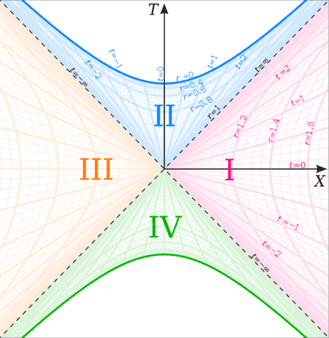
(Note that the coordinates in the diagram are scaled so that $2M = 1$, i.e., $r = 1$ is the boundary surface that we were calling $r = 2M$ in previous articles. I’ll continue to refer to this surface as $r = 2M$ here.)

In this article, we’re going to go into more detail about what this diagram tells us.

The first thing to note is that, unlike the spacetime diagrams we’re used to from Minkowski spacetime, this diagram does not cover the full range of the coordinates $T$ and $X$. Instead, there are two boundaries, marked by the hyperbolas $T^2 – X^2 = 1$, and coordinate values at or outside these boundaries are not part of the spacetime. These boundaries correspond to $r = 0$. (We’ll go into why there are two of them below.) If we look at the metric above, we can see that the coefficients of $dT^2$ and $dX^2$ diverge at $r = 0$, so our coordinates break down there. But we have seen that before, in Schwarzschild coordinates, and it turned out to be just an artifact of the coordinates. Is that the case here?

The way to tell, of course, is to look for invariants. Unfortunately, the simplest scalar invariant in curved spacetime, the Ricci scalar $R$, doesn’t help, because, in a vacuum spacetime, which this is, it is zero everywhere. But there is another scalar called the Kretschmann scalar, which is defined as $R^{abcd} R_{abcd}$, i.e., the full contraction of the Riemann tensor with itself. This scalar is not zero in Schwarzschild spacetime; its value is:

$$
K = \frac{48 M^2}{r^6}
$$

As you can see, this scalar diverges as $r \rightarrow 0$ (whereas it is finite at $r = 2M$, where we had the coordinate issue in Schwarzschild coordinates). So the boundary at $r = 0$ is not just an artifact of coordinates: it is a genuine “stopping point”, where the physical model of GR breaks down because the curvature of spacetime is no longer well-defined. (Of course, this means we don’t actually know what happens at this point–we only know that GR can’t tell us. One of the things we hope to get from a theory of quantum gravity, if and when we find it, is an answer to what happens at this point. But that will have to wait for a separate article. Here will assume that the GR model holds for all $r > 0$.)

The next thing we notice is that the two boundary hyperbolas are spacelike (because their slope is always less than 45 degrees). That means that they are best viewed, intuitively, as moments of time, not places in space. For example, the “future singularity” (the upper hyperbola) is a moment of time that is to the future of all events inside the black hole (the region marked II on the diagram). This is why, if you fall into region II, you can’t avoid reaching the singularity: for the same reason you can’t avoid reaching tomorrow. So we have to discard all intuitions about the singularity being a “place” that is “inside” the black hole.

In fact, we have to discard more intuitions than that. Consider the origin of the diagram: the point $T = 0$, $X = 0$. Our diagram has discarded two spatial dimensions, so each point on the diagram (in the region where it is valid, i.e., inside the two boundary hyperbolas) actually represents a 2-sphere with radius $r$, where $r$ is a function of $T$ and $X$ as discussed in the last article. So the origin of this diagram represents a 2-sphere with $r = 2M$ (or physical area $16 \pi M^2$).

Think about what this means. If this were an ordinary Minkowski diagram, the origin would represent a single event; even if we take into account that the diagram leaves out two spatial dimensions, putting them back would just make the origin a point in 4 dimensions instead of two–it would be a single event on the worldline of an observer sitting at the center of the spatial coordinates. But in the Kruskal-Szekeres diagram, the origin is not like that: it’s not a point, and it’s certainly not a “point at the center” of anything (because $r \neq 0$ there). It’s a 2-sphere.

Let’s probe this further by looking at the spacelike hypersurface $T = 0$. Note that this is also a spacelike hypersurface with Schwarzschild coordinate time $t = 0$. (It is not, however, a hypersurface of Gullstrand-Painleve coordinate time $T = 0$.) What does this hypersurface look like? Think of it in terms of 2-spheres: we start at the right, $X \rightarrow \infty$, where $r \rightarrow \infty$, so we have 2-spheres of larger and larger radius (or area). As we approach the origin $X = 0$, the 2-sphere radius (area) gets smaller, until at $X = 0$ it is $2M$. Then, as we move to the left, to negative values of $X$, the radius/area increases again! As $X \rightarrow – \infty$, we have $r \rightarrow \infty$ again, so the 2-sphere radii/areas increase without bound.

In other words, this spacelike hypersurface is an infinite family of 2-spheres that does not have a center; there is no 2-sphere with zero radius/area, as there would be in a spacelike hypersurface in Minkowski spacetime. In more technical language, the topology of this spacelike hypersurface is $S^2 times R$, not $R^3$. And the topology of the spacetime as a whole, since it is just an infinite family of such hypersurfaces, is $S^2 \times R^2$, not $R^4$ (the topology of Minkowski spacetime). This kind of spacelike hypersurface is unlike anything we ordinarily experience, and we have to discard many of our ordinary intuitions about “space” if we want to try to understand it.

One way of visualizing the geometry of this hypersurface is to put back one angular dimension. Then we have an infinite family of circles, going from infinite radius down to a radius of $2M$ and back to infinite radius again. This is the “wormhole” (or Einstein-Rosen bridge) that is often talked about in connection with this geometry. It is important to realize, though, that only the circles themselves–the surface of the “wormhole” shape–represent the spacelike hypersurface; the “inside” of the wormhole shape does not represent anything.

Another limitation of the “wormhole” visualization is that it is impossible for anything to actually travel through the wormhole. Looking at the spacetime diagram, we can see that there are no timelike or null paths that go from region I (the “right wedge”) to region III (the “left wedge”). All such paths are spacelike. This is sometimes described as the wormhole “pinching off” before anything can travel through it; this interpretation comes from looking at surfaces of constant $T$ from the bottom to the top of the diagram. These surfaces start out as two disconnected pieces, which then get connected by the wormhole, which increases from zero radius (at the bottom hyperbola) to radius $2M$ (at the origin), then decreases back to zero radius (at the top hyperbola), and the surfaces then split back into two disconnected pieces. Anyone in region I who tries to go through the wormhole as it opens up will find that he can’t make it into region III; he ends up stuck in region II and hits the future singularity.

Going back to the hypersurface through the origin, we can see something else: all of the spacelike hypersurfaces of constant Schwarzschild coordinate time $t$ have the same geometry, and they all intersect at the origin. This gives us another way of seeing what goes wrong with Schwarzschild coordinates at $r = 2M$: what time coordinate $t$ do we assign to the origin of our diagram? There is no well-defined answer. In fact, Schwarzschild coordinates are not a single coordinate chart on this spacetime; each of the four regions, I, II, III, and IV, has its own Schwarzschild coordinate chart, disconnected from all the others. (The line element has the same form in all four.)

This naturally leads to the question, what about Gullstrand-Painleve coordinates? They obviously cover region I, and we saw in the last article that they also cover region II, and are connected at the boundary between them (the portion of the $r = 2M$ line above and to the right of the origin) since they are well-defined at $r = 2M$. But do they cover anything else?

We can approach this question by considering the worldline of a freely falling object that, at some instant of time which we will label with Gullstrand-Painleve coordinate time $T = 0$, is at rest at a finite value of $r$ in region I (i.e., $r > 2M$). This object will free-fall into the black hole (region II), reaching the horizon $r = 2M$ at some finite $T > 0$, and reaching the singularity at $r = 0$ at some larger finite positive $T$. But what if we trace its worldline backward, to negative values of $T$? What we will find is that, no matter how negative $T$ gets, the worldline never reaches $r = 2M$; it just approaches it asymptotically, in much the same way that $r$ approached $2M$ asymptotically in Schwarzschild coordinates for $t \rightarrow \infty$.

Aided by our spacetime diagram, we can see what must be going on here. Gullstrand-Painleve coordinates–at least the ones we wrote down (we’ll see in a minute why I put in this qualifier)–only cover regions I and II. In these coordinates, $T \rightarrow – \infty$ corresponds to the lower boundary of region I, the one between regions I and IV. (We can also determine that these coordinates don’t cover region III either; in region II, $T \rightarrow – \infty$ for $r < 2M$ corresponds to the boundary between region II and region III.) So there seems to be an asymmetry in Gullstrand-Painleve coordinates which isn’t there in Schwarzschild coordinates.

The word “asymmetry” gives us a clue: what about the off-diagonal term in the metric? Notice that it has a $+$ sign in front of it. That is an asymmetry. What if we change it to a minus sign? That is, what if we consider this line element:

$$
ds^2 = – \left( 1 – \frac{2M}{r} \right) dT^2 – 2 \sqrt{\frac{2M}{r}} dT dr + dr^2 + r^2 \left( d\theta^2 + \sin^2 \theta d\phi^2 \right)
$$

If you check, you will see that with this line element, the time coordinate $T$ corresponds to the proper time for an observer who is free-falling outward, with increasing $r$, but decelerating, asymptotically approaching rest as $r \rightarrow \infty$. The coordinate speed of this observer is $dr / dT = \sqrt{2M / r}$ (note that three is no minus sign). Such an observer has a worldline that originates at the past singularity–the bottom hyperbola in our spacetime diagram–free-falling outward with $dr / dT \rightarrow \infty$, passing through region IV and through its boundary at $r = 2M$ into region I, with $dr / dT = 1$ at $r = 2M$ and decreasing. And there will also be worldlines that originate at the past singularity and free-fall outward, pass through $r = 2M$ into region I, but come to rest at some finite $r$–and then fall back into region II. In this new coordinate chart, we can only follow such worldlines up to the boundary with region II; $T \rightarrow \infty$ in this chart corresponds to $r \rightarrow 2M$ in the upper part of region I.

In other words, there are multiple Gullstrand-Painleve coordinate charts, just as there are multiple Schwarzschild coordinate charts; but the Gullstrand-Painleve charts each cover two regions, not one. The original Gullstrand-Painleve chart, the one we wrote down in previous articles, is called the “ingoing” chart, and covers regions I and II; and the new chart we wrote down above is called the “outgoing” chart and covers regions IV and I. (I have never seen it discussed, but it seems evident that there should also be two more such charts, an “ingoing” one that covers regions III and II, and an “outgoing” one that covers regions IV and III. Similar remarks would apply to Eddington-Finkelstein coordinates, which we haven’t discussed in this article but which are often encountered in discussions of this spacetime geometry.)

So we can see that the Kruskal-Szekeres spacetime diagram helps to fit together all the different charts on the Schwarzschild geometry, and gives us a consistent overall picture that we can visualize. But there is still one more intuition that we have to discard, in particular for the “interior” regions (II and IV), the ones between the event horizon at $r = 2M$ and the singularities at $r = 0$. Remember that curves of constant $r$ are hyperbolas, and they each cover an infinite range (of either the Schwarzschild $t$ or the Gullstrand-Painleve $T$, it doesn’t matter which one we look at for this purpose). In the “exterior” regions (I and III), these curves are timelike, so it’s easy to interpret them as the worldlines of a family of observers, each “hovering” at a constant altitude above the horizon, and existing for an infinite time.

However, in the interior regions, the curves of constant $r$ are spacelike. But nothing else has changed: they still cover an infinite range, and they are still integral curves of a Killing vector field, so the metric is unchanged along each of them. In other words, these curves, when we add back the two angular dimensions, each describe a spacelike hypersurface with a uniform geometry that is infinite in extent–yet somehow they all fit inside $r = 2M$! Clearly, the interior regions are quite unlike anything in our ordinary experience. (And to bend your head even further, consider that in Gullstrand-Painleve coordinates, surfaces of constant $T$ are spacelike all the way down to $r = 0$, and each one of them has only a finite extent in the interior region $r < 2M$. So the interior region has “spaces” that are finite and “spaces” that are infinite.)

We have covered the main points that we can learn from the spacetime diagram in Kruskal-Szekeres coordinates. But we still haven’t talked about a key question: how much of this spacetime geometry is actually physically relevant? We’ll go into that in the next article.

References

(1) The Wikipedia article on Kruskal-Szekeres coordinates, from which the spacetime diagram is taken:

Wikipedia article on Kruskal-Szekeres coordinates

The image was authored by Dr Greg, Wikimedia Commons (yes, the PF Science Advisor DrGreg).

(2) The Creative Commons License:

Creative Commons License