The Schwarzschild Metric: GPS Satellites

 

A Global Positioning System (GPS) device gives your precise location by receiving light pulses from satellites with synchronized clocks then triangulating your location based on that information [1]. Since light travels at 300 million meters per second, your location will be off by about 1 meter if the clock times are off by only 3 nanoseconds. Thus, extreme accuracy is absolutely necessary. As it turns out though, the satellite clocks in orbit run at a different rate than ground-based clocks due to a general relativistic effect. As Ashby points out [1], “If these relativistic effects were not corrected for, satellite clock errors building up in just one day would cause navigational errors of more than 11 km, quickly rendering the system useless.” In this Insight, I want to provide an overview of the general relativity (GR) calculations for this claim.

I begin with the Schwarzschild metric for the empty spacetime region surrounding the worldtube of a spherically-symmetric mass $M$ as derived in another Insight A Short Proof of Birkoff’s Theorem:

\begin{equation} ds^2 = -\left(1 – \frac{2M}{r}\right)dt^2 + \left(1 – \frac{2M}{r}\right)^{-1}dr^2 + r^2d\theta^2 + r^2 \sin^2\theta d\phi^2   \label{metric} \end{equation}

where we’re using units of $G = c = 1$ (I will occasionally restore $G$ and/or $c$ when convenient). Let’s review what the coordinates mean physically. First, we see that at $r = \infty$ Eq(\ref{metric}) is just the Minkowski metric in spherical coordinates, i.e., the flat spacetime of special relativity (SR). Thus, for an observer with constant spatial coordinates far from the spherically-symmetric mass $M$, proper time $\tau$ is coordinate time $t$ since $ds^2 = -d\tau^2$ on timelike worldlines and Eq(\ref{metric}) tells us $ds^2 = -dt^2$ at $r = \infty$ with $dr = d\theta = d\phi = 0$. So, now we know that the coordinate $t$ is the proper time for observers far from, and at rest with respect to, $M$. Next, let’s look at $r$. As pointed out in the Insight The Schwarzschild Geometry: Part 1, the radial coordinate is defined by the area of a sphere concentric with $M$. You might imagine measuring this area by making sure $M$ subtends a constant solid angle during the measurement process, that ensures you’ve measured the area of a sphere concentric with $M$. Any given sphere can then be given the standard polar and azimuthal coordinates $\theta$ and $\phi$, respectively, as usual. Once you’ve measured the area $A$ of the sphere at your location, you obtain your radial coordinate using $r^2 = \frac{A}{4\pi}$. Notice that the distance from $r_1 = 1$ and $r_2 = 3$, say, is not simply $r_2 – r_1 = 2$, but is larger according to the integral:

\begin{equation} \int\limits_{r_1}^{r_2} \frac{dr}{\sqrt{\left(1 – \frac{2M}{r}\right)}} \label{Rintegral} \end{equation}

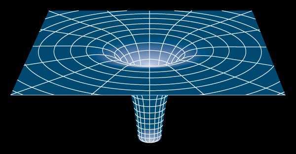
To show how concentric spheres in the space of Schwarzschild spacetime are spaced farther apart than their flat space counterparts, one often sees circles replacing spheres on a cone:

Now that we understand the coordinates for our metric and spacetime, we can proceed to ask and answer questions regarding various physical situations. In this Insight, I will compute the difference between clock rates for observers in geodetic orbit about $M$ (e.g., GPS satellites) and observers on the surface of $M$. Let’s start with the latter.

An observer on the surface of $M$ has a fixed radial coordinate $R$, which I will call “the radius of $M$,” although we need to keep in mind how the radial coordinate is defined. For this observer Eq(\ref{metric}) tells us that

\begin{equation} ds^2 = -d\tau_R^2 = -\left(1 – \frac{2M}{R}\right)dt^2  \label{RestObsTime1} \end{equation}

so that

\begin{equation} \Delta\tau_R = \sqrt{1 – \frac{2M}{R}}\Delta t  \label{RestObsTime2} \end{equation}

We see that time lapsed $\Delta\tau_R$ for the observer on $M$ is less than time lapsed $\Delta t$ for the observer far from, and at rest with respect to, $M$. For the observer in geodetic (free fall) orbit about $M$ with $\theta = 90^o$ and $r = r_o$ Eq(\ref{metric}) gives:

\begin{equation} ds^2 = -d\tau_o^2 = -\left(1 – \frac{2M}{r_o}\right)dt^2 + r_o^2 d\phi^2   \label{OrbitObsTime1} \end{equation}

so that

\begin{equation} \Delta\tau_o = \int\sqrt{1 – \frac{2M}{r_o} – r_o^2 \left(\frac{d\phi}{dt}\right)^2}\,dt   \label{OrbitObsTime2} \end{equation}

In order to do the integral in Eq(\ref{OrbitObsTime2}) we need to know $\frac{d\phi}{dt}$ for the geodetic orbit. We can get that from our four geodesic equations (one for each of our four coordinates):

\begin{equation} \frac{d^2 x^i}{d\tau^2} + \Gamma^i_{jk} \frac{dx^j}{d\tau}\frac{dx^k}{d\tau} = 0   \label{GdscEq} \end{equation}

where repeated upper and lower indices imply a sum over ${0, 1, 2, 3}$, our coordinates are $x^0 = t, x^1 = r, x^2 = \theta, x^3 = \phi$ and $\Gamma^i_{jk}$ are the Christoffel symbols (of the second kind):

\begin{equation} \Gamma^i_{jk} = \frac{g^{is}}{2}\left( \frac{\partial g_{sj}}{\partial x^k} + \frac{\partial g_{sk}}{\partial x^j} – \frac{\partial g_{jk}}{\partial x^s} \right) \label{Christoffel} \end{equation}

where $g^{is}$ is the inverse metric and again the repeated index $s$ implies a sum ${0, 1, 2, 3}$. For the metric components we have $g_{00} = -\left(1 – \frac{2M}{r}\right)$ and $g^{00} = -\left(1 – \frac{2M}{r}\right)^{-1}$, for example. Of the four geodesic equations, only $x^i = r$ is of any help and that gives us:

\begin{equation} \Gamma^1_{00} \frac{dt}{d\tau}\frac{dt}{d\tau} + \Gamma^1_{33} \frac{d\phi}{d\tau}\frac{d\phi}{d\tau} = 0   \label{GdscEq2} \end{equation}

having kept only the non-vanishing terms. Eq(\ref{Christoffel}) gives us:

\begin{equation} \Gamma^1_{00} = \frac{M}{r_o^2}\left(1 – \frac{2M}{r_o}\right) \label{ooChristoffel} \end{equation}

and

\begin{equation} \Gamma^1_{33} = -r_o\left(1 – \frac{2M}{r_o}\right) \label{33Christoffel} \end{equation}

Putting these into Eq(\ref{GdscEq2}) gives us:

\begin{equation} r_o\left(1 – \frac{2M}{r_o}\right)\left(\frac{d\phi}{d\tau}\right)^2 = \frac{M}{r_o^2}\left(1 – \frac{2M}{r_o}\right)\left(\frac{dt}{d\tau}\right)^2  \label{GdscEq3} \end{equation}

We can reject the $r_o = 2M$ solution since the Schwarzschild metric is only valid outside of $M$ and $r = 2M$ is about 1 cm for $M$ the mass of Earth, i.e., well inside Earth! That means

\begin{equation} \left(\frac{d\phi}{dt}\right)^2 = \frac{M}{r_o^3}  \label{GdscEq4} \end{equation}

which looks very Newtonian, i.e., $\frac{v^2}{r} = \frac{GM}{r^2}$ where $v = \omega r$ and $\omega = \frac{d\phi}{dt}$ (as pointed out in The Schwarzschild Geometry: Part 1). The difference is that in GR $t$ is proper time only for distant stationary observers while there is only one proper time for all observers in Newtonian physics. Plugging Eq(\ref{GdscEq4}) into Eq(\ref{OrbitObsTime2}) we obtain:

\begin{equation} \Delta\tau_o = \sqrt{1 – \frac{3M}{r_o}}\, \Delta t  \label{OrbitObsTime3} \end{equation}

Notice that the observer on $M$ will measure a shorter time lapse for a given $\Delta t$ than the orbiting observer as long as $r_o > 1.5R$. If it wasn’t for that third term $- r_o^2 \left(\frac{d\phi}{dt}\right)^2$ in Eq(\ref{OrbitObsTime2}), i.e., the “$-\frac{v^2}{c^2}$” term, the orbiting clock would run faster than the $M$-based clock for any $r_o$. So, as is sometimes mentioned in popular presentations of SR, there is an “SR time dilation effect” for orbiting objects. This “SR effect” dominates at $r_o < 1.5R$ so that the orbiting clock actually runs slower than the $M$-based clock for such low-altitude orbits.

Of course, the GPS satellites orbit at a much higher altitude than $1.5 R_{Earth}$, so they run faster than Earth-based clocks. As Ashby points out [1], the GPS satellites have orbital periods of 11 hr 58 min (half a sidereal day) which means (using Kepler’s third law) they have an orbital radius of 26,600 km. Using the orbital radius, Earth radius and Earth mass in Eq(\ref{RestObsTime2}) & Eq(\ref{OrbitObsTime3}) tells us that the GPS satellite clocks run faster than the Earth-based clocks by 4.46 parts per 10 billion. Thus, over the course of one day (two orbits) the time difference is 38.4 $\mu$s and in that amount of time light travels 11.5 km, as claimed by Ashby.

Of course, as pointed out by PeterDonis, this neglects the rotation of Earth. One might think we should use the Kerr metric rather than the Schwarzschild metric, since the Kerr metric represents an axisymmetric space rather than a spherically symmetric space. However, “The Kerr metric does not represent the exterior metric of a physically likely source, nor the metric during any realistic gravitational collapse” [2]. The reason for this is that there is no known interior (matter) solution that adjoins the Kerr exterior solution (metric). On the other hand, the Schwarzschild metric does join to spherical matter distributions with and without pressure (one can join it to an expanding or collapsing, dust-filled FLRW metric for example [3]), so I’ll use it to approximate Earth’s rotational effect on Eq(\ref{RestObsTime2}). We need only add the “$-\frac{v^2}{c^2}$” term as in Eq(\ref{OrbitObsTime2}), i.e., Eq(\ref{RestObsTime1}) now reads:

\begin{equation} ds^2 = -d\tau_R^2 = -\left(1 – \frac{2M}{R}\right)dt^2 + R^2 \sin^2\theta d\phi^2  \label{RestObsTime3} \end{equation}

We have $\frac{v^2}{c^2} = \frac{R^2_{Earth} \sin^2(\theta)\omega^2}{c^2}$ where $\omega = 2\pi/day$ (ignoring the ambiguity between proper time and coordinate time for this estimate). This term is of order $10^{-12}$ while the term $\frac{2GM}{c^2R}$ is of order $10^{-9}$, so I have ignored the rotation of Earth for computing the time differences (see Ashby [1] for that analysis).

References

1. Ashby, N.: Relativity and the global positioning system. Physics Today 55(5), 41–47 (2002).
2. Teukolsky, S.: The Kerr Metric. Classical & Quantum Gravity 32, 124006 (2015).
3. Stuckey, W.M.: The observable universe inside a black hole. American Journal of Physics 62, 788-795 (1994).