Learn About the FLRW Metric and The Friedmann Equation

Previous Chapter: A Journey Into the Cosmos – The Friedmann Equation

               Chapter 2- FLRW Metric and The Friedmann Equation

In this chapter, we will further investigate the Friedmann equation and we will explore the FLRW metric. We will solve the Friedmann equation for three different types of models (matter-dominated, radiation-dominated, and mixed) and observe how the Universe evolves concerning these models.

          Part 1- Curved Space and The Metric

It would be better if we construct a basic idea about the curvature, before trying to understand the FLRW metric.

We claimed that isotropy and homogeneity reduce the possible spaces that can exist due to symmetry ^[1]. These possible geometries are;

  I. Flat space of zero curvature

 II. Three-dimensional sphere of positive constant curvature

III. Three-dimensional hyperbolic space of negative constant curvature

To understand the concept of curvature (also the FLRW metric) in a better way, let us start to examine these possibilities in two-dimensional space. Then we will extend our content to three and later on four dimensions to describe the FLRW metric.

       1.1 Two-Dimensional Space

  I. Flat space of zero curvature

In a Euclidean two-dimensional space, if we construct a triangle, the sum of angles of this triangle must be $π$

$$α+β+γ=π~~~~~(1.1)$$

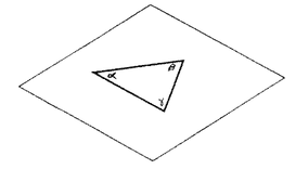          Fig.1: A flat two-dimensional space

Where the angles are measured in radians. If we satisfy this condition, we can say that the curvature of space is zero and it has a flat geometry.

In flat space, we can set a cartesian coordinate system and choose two points, $(x,y)$ and $(x+dx,y+dy)$  so that the distance $(ds)$  between two points will be

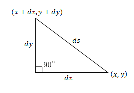
          Fig. 2: Measuring distance $(ds)$ in flat two-dimensional space

$$ds^2=dx^2+dy^2~~~~~(1.2)$$

Stating that equation $(1.2)$ holds everywhere in a two-dimensional space is equivalent to saying that space is a plane. Of course, other coordinate systems can be used, in place of cartesian coordinates. For instance, in polar coordinates, we can set two points, $(r,θ)$  and $(r+dr,θ+dθ)$  this time the distance $(ds)$ will be

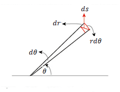
          Fig. 3: Measuring distance $(ds)$ in polar coordinates

$$ds^2=dr^2+r^2dθ^2~~~~~(1.3)$$

 

  II. Positively Curved Two-Dimensional Space

In a positively curved two-dimensional space, if we construct a triangle, the sum of angles of this triangle must be larger than $π$

$$α+β+γ=π+\frac {A} {R^2}~~~~~(1.4)$$

Where $A$ is the area of the triangle and $R$  is the radius of the sphere.

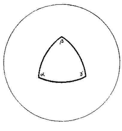
          Fig. 4: A positively curved two-dimensional space

All spaces in which  $α+β+γ>π$  are called “positively curved” spaces.

On the surface of a sphere, we can set up a polar coordinate system by picking a pair of antipodal points to be the “north pole” and “south pole” and by picking a geodesic from the north to the south pole to be the “prime meridian”. If $r$  is the distance from the north pole, and $θ$ is the azimuthal angle measured relative to the prime meridian, then the distance $(ds)$  between a point $(r,θ)$  and another nearby point $(r+dr,θ+dθ)$  is given by the relation

          Fig. 5: Measuring distance $(ds)$  in a positively curved two-dimensional space ^[2}

$$ds^2=dr^2+R^2sin^2(\frac {r} {R})dθ^2~~~~~(1.5)$$

  III. Negatively Curved Two-Dimensional Space

In a negatively curved two-dimensional space, if we construct a triangle, the sum of angles of this triangle must be less than $π$

$$α+β+γ=π-\frac {A} {R^2}~~~~~(1.6)$$

Where $A$  is the area of the triangle and $R$   is the radius of the curvature.

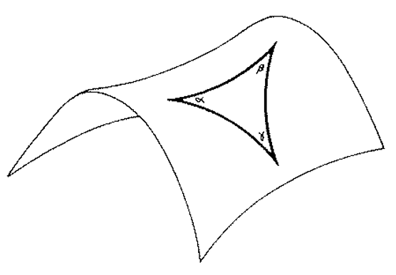
          Fig. 6: Negatively curved two-dimensional space

On a surface of constant negative curvature, we can set up a polar coordinate system by choosing some point as the pole, and some geodesic leading away from the pole as the prime meridian. If $r$ is the distance from the pole, and $θ$ is the azimuthal angle measured relative to the prime meridian, then the distance $(ds)$  between a point $(r,θ)$  and a nearby point $(r+dr,θ+dθ)$ is given by

$$ds^2=dr^2+R^2sinh^2(\frac {r} {R})dθ^2~~~~~(1.7)$$

Relations like those presented in equations $(1.3)$, $(1.5)$, and $(1.7)$ which give the distance $ds$ between two nearby points in space, are known as metrics. The metric can be thought of as a distance function that defines the distance between each pair of elements of a set ^[3]. In general, the curvature is a local property. A tablecloth can be badly rumpled at one end of the table and smooth at the other end; a bagel (or another toroidal object) is negatively curved on part of its surface and positively curved on other portions. However, if you want a two-dimensional space to be homogeneous and isotropic, there are only three possibilities that fit the bill: space can be uniformly flat, it can have uniform positive curvature, or it can have uniform negative curvature.

Thus, if a two-dimensional space has a curvature that is homogeneous and isotropic, its geometry can be specified by two quantities, $κ$, and $R$. The number $κ$, called the curvature constant, $κ=0$ for a flat space, $κ=+1$ for a positively curved space and $κ=-1$ for negatively curved space. If the space is curved, then the quantity $R$, which has dimensions of length, is the radius of curvature.

       1.2 Three-Dimensional Space

The metric for $κ=1,0,-1$  in the two-dimensional case can be easily extended to three-dimension. In three-dimensional space

I. For $κ=0$ , in a cartesian coordinate system, the metric can be expressed by

$$ds^2=dx^2+dy^2+dz^2~~~~~(1.8)$$

or in polar coordinate system

$$ds^2=dr^2+r^2[dθ^2+sin^2θdφ^2]~~~~~(1.9)$$

II. For $κ=+1$ , the metric will be

$$ds^2=dr^2+R^2sin^2(\frac {r} {R})[dθ^2+sin^2θdφ^2]~~~~~(1.10)$$

III. For $κ=-1$ , the metric will be

$$ds^2=dr^2+R^2sinh^2(\frac {r} {R})[dθ^2+sin^2θdφ^2]~~~~~(1.11)$$

These three possible metrics for a homogeneous, isotropic, three-dimensional space can be written more compactly in the form of

$$ds^2=dr^2+S_κ(r)^2dΩ^2~~~~~(1.12)$$

Where

$$dΩ^2=dθ^2+sin^2θdφ^2~~~~~(1.13)$$

And

 

$$S_κ(r)=\begin{cases}
Rsin(\frac {r} {R}) & κ=+1 \\
r & κ=0 \\
Rsinh(\frac {r} {R})& κ=-1
\end{cases}~~~~~(1.14)$$

The coordinate system $(r,θ,φ)$ is not the only possible system. For instance, if we switch the radial coordinate from $r$ to $x≡S_κ(r)$, the metric for a homogeneous, isotropic, three-dimensional space can be written as

$$ds^2=\frac {dx^2} {1-κ\frac {x^2}{R^2}}+x^2dΩ^2~~~~~(1.15)$$

Curvature Constant $(κ)$	Type of Universe	Angles of Triangle	Metric Equation
$-1$	Open	$<π$	$ds^2=dr^2+R^2sinh^2(\frac {r} {R})dΩ^2$
$0$	Flat	$π$	$ds^2=dr^2+r^2dΩ^2$
$+1$	Closed	$>π$	$ds^2=dr^2+R^2sin^2(\frac {r} {R})dΩ^2$

         

          Part 2- FLRW metric

Now we can pass to four dimensions and try to understand the FLRW metric.

Let’s consider two events, one of them in $(t,r,θ,φ)$  and the other one is in $(t+dt,r+dr,θ+dθ,φ+dφ)$.

Then, according to special relativity, the space-time separation will be

$$ds^2=-c^2dt^2+dr^2+r^2dΩ^2~~~~~(2.1)$$

This is the Minkowski metric, and it applies to a case where the space-time is flat, and curvature is zero.

So, here we can ask “What form can the metric of space-time assume if the Universe is spatially homogeneous and isotropic at all time and if distances are allowed to expand (or contract) as a function of time?”

The FLRW metric gives us an answer to this question, it can be written as

$$ds^2=-c^2dt^2+a^2(t)[\frac {dx^2} {1-κ\frac {x^2}{R^2}}+x^2dΩ^2]~~~~~(2.2)$$

We can notice that there is a scale factor in this equation which, represents how proper distance changes with time. Also, the spatial metric component of the FLRW metric consists of the spatial metric for a uniformly curved space of radius $(Eqn. (1.15))$. The FLRW metric is a spatial curvature of the Universe, not a space-time curvature.

FLRW metric can be also written as

$$ds^2=-c^2dt^2+a^2(t)[dr^2+S_κ(r)^2dΩ^2]~~~~~(2.3)$$

(See equation $(1.12)$ and $(1.14)$)

The time variable  $t$ in the FLRW metric is the cosmological proper time called the cosmic time for short and is the time measured by an observer who sees the Universe expanding uniformly around him. The spatial variables $(x,θ,φ)$ or $(r,θ,φ)$ is called the comoving coordinates. If the expansion of the Universe is perfectly homogeneous and isotropic, the comoving coordinates of any point remain constant with time.

In this equation, we can see that there are three things that are important for us to determine the geometry and hence the true description of the metric of the Universe, these are $κ$, $R$, and $a(t)$.

       2.1 Proper Distance        

Now we can try to find the proper distance using the FLRW metric. We defined the FLRW metric as

$$ds^2=-c^2dt^2+a^2(t)[dr^2+S_κ(r)^2dΩ^2]$$

In an expanding universe, the distance between objects increases with time. Thus, if we want to assign a spatial distance between two objects, we should specify a time $t$, which the distance is the correct one.

The proper distance $(d_p(t))$ between two points is equal to the length of the spatial geodesic between them when the scale factor is fixed at the value $a(t)$.

Suppose we are at the origin $(0,0,0)$, and the galaxy that we are observing has a comoving coordinate of $(r,θ,φ)$.

In the FLRW metric, since we fixed the time,  $-cdt^2$ terms become zero.

$$ds^2=a^2(t)[dr^2+S_κ(r)^2dΩ^2]~~~~~(2.4)$$

Also, along this spatial geodesic between the observer and galaxy, the angle $(θ,φ)$ becomes constant

$$dΩ^2=dθ^2+sin^2θdφ^2=0~~~~~(2.5)$$

Thus

$$ds^2=a^2(t)[dr^2]$$

$$ds=a(t)dr~~~~~(2.6)$$

Now we can define the proper distance by integrating over the radial comoving coordinate $r$

$$d_p(t)=a(t)\int_0^r  \, dr=a(t)r~~~~~(2.7)$$

It’s the same equation that we find in the first chapter of the article (I used $Δx$ instead of $r$). Since we obtain the proper distance equation, from here we can derive Hubble’s Law ^[4].

       2.2 Cosmological Redshift

When we observe the sky, all information comes from the light emitted from distant objects. This emitted light travels through space-time, since it has a finite speed and the Universe expands, the wavelength of the light changes due to this expansion and we call it the cosmological redshift.

          Fig. 7: Cosmological Redshift ^[5]

We know that each element emits photon only at a certain wavelength and by comparing this wavelength with the measured one from the distant objects, we can determine the value of the redshift.

$$z=\frac {λ_0-λ_e} {λ_e}=\frac{δλ}{λ}~~~~~(2.8)$$

Here, $z$  is the redshift, $λ_0$ is the observed wavelength from the distant object, $λ_e$  is the emitted wavelength, and $δλ$ means a change in the wavelength.

  I. Cosmological Redshift and The Expansion

Cosmological redshift is a very useful tool to calculate the rate of expansion since the expansion causes redshift. We can find this relationship using the FLRW metric.

Let’s re-write the FLRW metric

$$ds^2=-c^2dt^2+a^2(t)[dr^2+S_κ(r)^2dΩ^2]~~~~~(2.9)$$

We know that for a light, $ds^2=0$, $θ=0$  and $φ=0$. Also when the light emitted, $t=t_e$ , $r=r_e$ and when it’s observed, $t=t_0$, $r=r_e=0$. Thus

$$0=-c^2dt^2+a^2(t)dr^2$$

$$\frac {cdt} {a(t)}=-dr~~~~~(2.10)$$

We have chosen the negative sign since both $a(t)$ and $t$ increase to the future, whereas $r$ increases away from the observer.

Now let’s take integral for both sides of the equation,

$$\int_{t_e}^{t_0} \frac {c} {a(t)}  \, dt=-\int_{r_e}^{r_0} \, dr$$

$$\int_{t_e}^{t_0} \frac {c} {a(t)}  \, dt=\int_{r_0=0}^{r_e=r} \, dr=r~~~~~(2.11)$$

Let’s concentrate on a particular wave crest of light, that was emitted at time $t_e$ (which is described by equation $(2.11)$). The next wave crest will be emitted at, $t_e+\frac {λ_e} {c}$ and it will observed at, $t_0+\frac {λ_0} {c}$. Hence, for the second wave crest, we can write,

$$\int_{t_e+\frac {λ_e} {c}}^{t_0+\frac {λ_0} {c}} \frac {c} {a(t)}  \, dt=\int_{r_0=0}^{r_e=r} \, dr=r~~~~~(2.12)$$

From $(2.12)$ and $(2.11)$ we can write,

$$\int_{t_e}^{t_0} \frac {c} {a(t)}  \, dt=\int_{t_e+\frac {λ_e} {c}}^{t_0+\frac {λ_0} {c}} \frac {c} {a(t)}  \, dt~~~~~(2.13)$$

If we subtract both sides of the equation with

$$\int_{t_e+\frac {λ_e} {c}}^{t_0} \frac {c} {a(t)}  \, dt$$

We get

$$\int_{t_e}^{t_e+\frac {λ_e} {c}}  \frac {c} {a(t)}  \, dt=\int_{t_0}^{t_0+\frac {λ_0} {c}}  \frac {c} {a(t)} \, dt~~~~~(2.14)$$

The $a(t)$ difference will be extremely small between two wave crests. Hence, we can assume it’s constant. Thus

$$\frac {1} {a(t_e)} \int_{t_e}^{t_e+\frac {λ_e} {c}}  \, dt=\frac {1} {a(t_0)} \int_{t_0}^{t_0+\frac {λ_0} {c}}  \, dt~~~~~(2.15)$$

And that is equal to

$$\frac {λ_e} {a(t_e)}=\frac {λ_0} {a(t_0)}~~~~~(2.16)$$

And we know that

$$z=\frac {λ_0-λ_e} {λ_e}=\frac{δλ}{λ}=\frac {λ_0} {λ_e}-1~~~~~(2.17)$$

Hence, using $(2.16)$ and $(2.17)$ we can write

$$z+1=\frac {λ_0} {λ_e}=\frac {a(t_0)} {a(t_e)}~~~~~(2.18)$$

We can choose $a(t)=1$  (It’s a convention which, describes the scale factor as $1$ for now).

For last, we can write

$$z+1=\frac {1} {a(t_e)}~~~~~(2.19)$$                                                                                                                                                                                                                                                                                                                                                    

This equation perfectly describes the relationship between redshift and the scale factor. Lets suppose we calculated redshift as $3$ , hence

$$3+1=\frac {1} {a(t_e)}~→~a(t_e)=\frac {1}{4}$$

This means that when the object emitted the light the Universe was $\frac {1} {4}$ times smaller than now. We should remember that the redshift we observe for a distant object depends only on the relative scale factors at the time of emission and the time of observation ^[6].

          Part 3- The Fluid Equation

The fluid equation has an important place in understanding the Friedmann equation. We described the Friedmann equation as

$$H^2=\frac {8πG} {3}ρ-\frac {κ} {a^2(t)}~~~~~(3.1)$$

If we look at the equation we will see that there are only two time-dependent variables; $a(t)$ and $ρ$. Hence, it’s important to understand how the density of the material in the Universe evolves with time.

To derive the relationship between $a(t)$ and $ρ$, we can use the fluid equation.

Let’s start with the first law of thermodynamics;

$$dE+PdV=dQ~~~~~(3.2)$$

Where, $dQ$ is the heat flow into or out of a region, $dE$ is the change in the internal energy, $P$ is the pressure, and $dV$ is the change in the volume of the region.

Here $dQ$ term will be zero because the Universe is an adiabatic system, which means there’s no place for “heat” to come from (so that the change in heat $(dQ)$  must be zero). In an adiabatic system all energy transfers to work. Hence, our equation becomes

$$dE+PdV=0~→~\dot E+P\dot V=0~~~~~(3.3)$$

For a comoving radius $r_s$ , we can write the volume as,  $V=\frac {4} {3}πr^3a^3(t)$, Thus

$$\dot V=4πr^3a^2(t)\dot {a}(t)=3V(\frac {\dot {a}(t)} {a(t)})~~~~~(3.4)$$     

And energy density, $ρ=\frac {E}{V}~→~E=ρV$, where

$$\dot E=\dot {ρ}V+ρ\dot {V}=V(\dot ρ+3ρ(\frac {\dot {a}(t)} {a(t)})~~~~~(3.5)$$

Using $(3.3)$ we can write

$$V(\dot {ρ}+3ρ(\frac {\dot {a}(t)} {a(t)})+3P(\frac {\dot {a}(t)} {a(t)})=0~~~~~(3.6)$$

Thus

$$\dot {ρ}+3(\frac {\dot {a}(t)} {a(t)})(ρ+P)=0~~~~~(3.7)$$

This is the fluid equation and it describes the evolution of energy density in an expanding universe. But to solve this equation we need an additional equation that states the relationship between $P$ and $ρ$.

However, before describing that equation, I want to make a point on the concept of density ^[7].

       3.1 Describing the Density

Let’s try to understand the density concept for different types of materials in the Universe, in this case for matter and radiation.

  I. Matter Density

Let’s think a region on large scales, approximately $100Mpc$, where the Universe is almost homogeneous and isotropic. A region with the volume of $R_xR_yR_z$ and a mass of $M$.

Hence the matter density of this region will be

$$ρ_m=\frac {M} {R_xR_yR_z}~~~~~(3.8)$$

From the previous chapter we learned that in comoving coordinate system, proper distance can be defined as

$$R_x=a(t)Δx~~~R_y=a(t)Δy~~~R_z=a(t)Δz~~~~~(3.9)$$

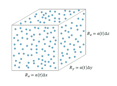
     Fig. 8: A region of the Universe where it contains $n$ number of galaxies, whose total mass of the galaxies are $M$ ( $\sum_{i=1}^n m_i =M$, where $m_i$  is the mass of the each galaxy).

Let’s insert $(3.9)$ into $(3.8)$

$$ρ_m=\frac {M}{a^3(t)ΔxΔyΔz}~~~~~(3.10)$$

We can set a new parameter $ν$ which it can be defined as a mass per cubic delta $(Δ)$  volume

$$ν=\frac {M} {ΔxΔyΔz}~~~~~(3.11)$$

It’s a constant value and it depends on the chosen region.

Hence, we obtain

$$ρ_m=\frac {υ} {a^3(t)}~~~~~(3.12)$$

As an alternative, we can simply say $ρ_m∝\frac {1} {a^3(t)}$

II. Radiation Density

To understand the idea of radiation density, we can consider a box filled with radiation. The first thing we should notice is that in the radiation case, we can talk about radiation energy density. We know that the radiation energy and wavelength are inversely proportional.

$$E∝\frac {1} {λ}~~~~~(3.13)$$

The volume of the box is proportional to $a^3(t)$ and we should assume that the wavelength of the box is also readjusted their wavelength to the size of the box.

$$E∝\frac {1} {a(t)}~~~~~(3.14)$$

     Fig. 9: The wavelength adjusts itself with respect to the size of the box ^[8]

Hence the radiation energy density can be defined as

$$ρ_r=\frac {E} {V}=\frac {\frac {C} {a(t)}} {a^3(t)}=\frac {C} {a^4(t)}~~~~~(3.15)$$

Here, $C$ is a constant number.  We can see that in the radiation case, the density decreases as $\frac {1} {a^4(t)}$ ^[9].

       3.2 Equation of State

Now we can study the relationship between $P$ and $ρ$. Let’s assume there is a linear relationship between $P$ and $ρ$.

$$P=ωρ~~~~~(3.16)$$

Where $ω$ is a constant number. Then from fluid equation $(3.7)$ we can write

$$\dot {ρ}+3(\frac {\dot {a}(t)} {a(t)})(ρ+ωρ)=0$$

$$\dot {ρ}+3ρ(\frac {\dot {a}(t)} {a(t)})(1+ω)=0$$

$$\frac {\dot {ρ}}{ρ}=-3(\frac {\dot {a}(t)} {a(t)})(1+ω)=0~~~~~(3.17)$$

Has a solution as

$$ρ=a(t)^{-3(1+ω)}~~~~~(3.18)$$

Which is called the equation of state.

As we see in Part 3.1, equation $(3.18)$ describes the density value for different types of materials in the Universe (means for different values of $ω$ ) ^[7].

Type of Material	Value of	Pressure	Density
Matter	$ω=0$	$P=ωρ=0$	$ρ=a(t)^{-3(1+0)}=\frac {1} {a^3(t)}$
Radiation	$ω=\frac {1} {3}$	$P=ωρ=\frac {ρ} {3}$	$ρ=a(t)^{-3(1+\frac {1}{3})}=\frac {1} {a^4(t)}$

 

       3.3 The Acceleration Equation

Since we described the fluid equation and the equation of state, we can combine these equations with the Friedmann equation.

The Friedmann equation is

$$H^2=\frac {8πG} {3}ρ-\frac {κ} {a^2(t)}~~~~~(3.19)$$

Let’s differentiate the equation with respect to $t$.

$$2H\dot {H}=\frac {8πG} {3}\dot {ρ}+\frac {2κ\dot {a}(t)} {a^3(t)}~~~~~(3.20)$$

Now, substituting $\dot {p}$ that we derived in $(3.7)$

$$\dot {ρ}+3(\frac {\dot {a}(t)} {a(t)})(ρ+P)=0~~~~~(3.7)$$

$$\dot {ρ}=-3(\frac {\dot {a}(t)} {a(t)})(ρ+P)$$

$$2H\dot {H}=\frac {8πG} {3}[-3(\frac {\dot {a}(t)} {a(t)})(ρ+P)]+\frac {2κ\dot {a}(t)} {a^3(t)}~~~~~(3.21)$$

We can cancel the $2H$ (where $H=\frac {\dot {a}(t)} {a(t)}$) from each term. Thus

$$\dot {H}=-4πG(ρ+P)+\frac {κ} {a^2(t)}~~~~~(3.22)$$

Or we can write as,

$$\dot {H}=\frac {\ddot {a}} {a}-(\frac {\dot {a}} {a})^2=-4πG(ρ+P)+\frac {κ} {a^2(t)}$$

Substituting $H^2$  (from $(3.19)$) in $(3.22)$

$$\frac {\ddot {a}} {a}-[\frac {8πG} {3}ρ-\frac {κ} {a^2(t)}]=-4πG(ρ+P)+\frac {κ} {a^2(t)}$$

$$\frac {\ddot {a}} {a}=-4πG(ρ+P)+\frac {κ} {a^2(t)}]-\frac {κ} {a^2(t)}]+\frac {8πG} {3}ρ$$

Finally, we derive

$$\frac {\ddot {a}} {a}=-\frac {4πG} {3}(ρ+3P)~~~~~(3.23)$$

Which is called the acceleration equation. The negative sign may seem strange or unexpected, but it makes sense (if there was a positive sign, that would mean that when you increase the density, the universe accelerates faster which doesn’t make any sense). In the equation, as you may see, increasing the density decelerates the expansion as expected.

Also in the acceleration equation as you may notice there’s no curvature constant. Which is canceled during the derivation of the equation ^[10].

       Part 4- The Friedmann Equation-Cosmological Models

In this part, we will try to solve the Friedmann equation for matter-dominated, radiation-dominated, and mixed universe models (only for the case of $κ=0$ ).

   I. Matter Dominated Universe

Let’s write the Friedmann equation

$$H^2=\frac {8πG} {3}ρ-\frac {κ} {a^2(t)}~~~~~(4.1)$$

For $κ=0$ , which represents a flat space, and for matter density $(ρ_m=\frac {1} {a^3(t)})$ we get

$$H^2=\frac {8πG} {3}ρ_m~~~~~(4.2)$$

$$(\frac {\dot{a}(t)} {a(t)})^2=\frac {8πG} {3a^3(t)}$$                                                                               

$$(\dot{a}(t))^2=\frac {8πG} {3a(t)}$$

And it has a solution as

$$a(t)=t^{\frac {2} {3}}~~~~~(4.3)$$

From there we can find the Hubble parameter

$$H=\frac {\dot {a}(t_0)}{a(t_0)}=\frac {2} {3t}~~~~~(4.4)$$

In this solution universe expands forever but the rate of expansion (Hubble parameter) decreases with time. Notice that despite the pull of gravity, the material in the Universe does not recollapse but rather expands forever.

   II. Radiation Dominated Universe

Let’s write the Friedmann equation

$$H^2=\frac {8πG} {3}ρ-\frac {κ} {a^2(t)}$$

For $κ=0$ , which represents a flat space, and for matter density $(ρ_r=\frac {1} {a^4(t)})$ we get

$$H^2=\frac {8πG} {3}ρ_r~~~~~(4.5)$$

$$(\frac {\dot{a}(t)} {a(t)})^2=\frac {8πG} {3a^4(t)}$$   

$$(\dot{a}(t))^2=\frac {8πG} {3a^2(t)}$$

It has a solution as

$$a(t)=t^{\frac {1} {2}}~~~~~(4.6)$$

But in this case, as we can notice universe expands more slowly than the matter-dominated case.

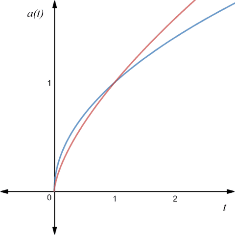
Fig. 10: Scale factor versus time.
(The blue line represents the radiation-dominated model while the red line is the matter-dominated

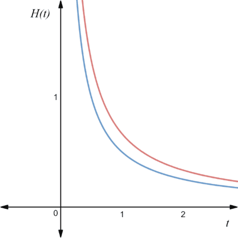
Fig. 11: Expansion rate versus time.
(The blue line represents the radiation-dominated model while the red line the matter-dominated)

 

 

 

 

 

 

 

 

 

 

 

 

There’s also something important to mention that, the scale factor does not mean anything by itself (in the case of expansion). For example, If I say $a(t)=20$, we can’t say anything about the process of expansion. Scale factor by itself just gives us the proper distance of an object at a given time $t$. Meanwhile, the ratios of the scale factor can give us a description of the evolution of the universe. We can see this ratio term in the redshift equation $(z+1=\frac {a(t_0)} {a(t_e)})$, in the Friedmann equation $(H^2=(\frac {\dot{a}(t)} {a(t)})^2)$ or in the acceleration equation  $(\frac {\ddot {a}} {a})$. This is why the Hubble parameter is important to understand the expansion of the universe or in other words the Friedmann equation.

As you can see in Fig. 10 even the $a(t)$ increases with time, $H$ decreases. But we should also notice that even $H$  decreases, it never becomes zero (only when, $\lim_{t \rightarrow +\infty} {H(t)}=0$ ).

We can see this effect both in radiation and matter-dominated cases (Fig. 11).

   III. Mixed (Matter+Radiation) Universe

In this case, I’ll not solve the exact equation, but I’ll make a general solution for this model.

In general, we can write the density in terms of its components

$$ρ=ρ_m+ρ_r~~~~~(4.7)$$

Where

$$ρ=\frac {1}{a^3(t)}+\frac {1}{a^4(t)}~~~~~(4.8)$$

Here we can see that when $a(t)<1$, the density contribution that comes from the radiation will be higher than matter. In other words, radiation density is more important to determine evolution. Hence, the Universe will evolve like $a(t)=t^{\frac {1} {2}}$.

But after a time when $a(t)>1$ matter density will be more important to determine the evolution of the universe. Hence, we can say that the universe will evolve like $a(t)=t^{\frac {2} {3}}$.

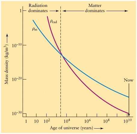
     Fig. 12: A schematic illustration of the evolution of a Universe containing radiation and matter. Once matter comes to dominate the expansion rate speeds up, so the densities fall more quickly with time ^[11].

Fig. 12 shows the evolution of a Universe containing matter and radiation, with the radiation initially dominating. Eventually, the matter comes to dominate, and as it does so the expansion rate speeds up from $a(t)=t^{\frac {1} {2}}$ to the $a(t)=t^{\frac {2} {3}}$. This may be the situation that applies in our present Universe ^[12].

       4.1 Critical Density

Let’s start with the Friedmann equation again

$$H^2=\frac {8πG} {3}ρ-\frac {κ} {a^2(t)}$$

For a given value of $H$, there is a special value of the density that would be required to make the geometry of the Universe flat, $κ=0$. This is known as the critical density $ρ_c$ , and it is given by

$$p_c(t)=\frac {3H^2} {8πG}~~~~~(4.9)$$

Critical density is a function of time because the Hubble parameter also changes with time.

Since we know the current Hubble parameter, we can calculate the critical density as

$$p_c(t_0)=1.88h^2×10^{-26}kg~m^{-3}$$

Where $h=0.72$

Be sure to understand that the critical density is not necessarily the true density of the Universe since the Universe need not be flat. However, it sets a natural scale for the density of the Universe. Consequently, rather than quote the density of the Universe directly, it is often useful to quote its value relative to the critical density. This dimensionless quantity is known as the density parameter $Ω$, defined by

$$Ω(t)=\frac {ρ} {ρ_c}~~~~~(4.10)$$

Where $ρ$ is the density value at a given time $t$.

Since the density parameter changes with time, the current density parameter is denoted by $Ω_0$. Where

$$Ω_0=\frac {ρ_0} {ρ_c}$$

In this case $ρ_0$ represents the current density value $(ρ_0=ρ_{now})$.

Our Universe contains several different types of matter, and this notation can be used not just for the total density but also for each component of the density like $Ω _{mat}$, $Ω _{rad}$.

In this case

$$ρ=ρ_m+ρ_r~~~~~(4.11)$$

Dividing both side of the equation with $ρ_c$

$$\frac {ρ} {ρ_c}=\frac {ρ_m+ρ_r} {ρ_c}=\frac {ρ_m} {ρ_c}+\frac {ρ_r} {ρ_c}~~~~~(4.12)$$

Hence, we can write

$$Ω=Ω _{mat}+Ω _{rad}~~~~~(4.13)$$

$Ω _{mat}=\frac {ρ_m} {ρ_c}=\frac {8πG}{H^2a^3}$, and for radiation, $Ω _{rad}=\frac {ρ_r} {ρ_c}=\frac {8πG}{H^2a^4}$^[13].

We can re-write the Friedmann equation, using the density parameter

$$H^2=\frac {8πG} {3}ρ-\frac {κ} {a^2(t)}$$

Dividing the equation by $ρ_c$

$$\frac {H^2} {ρ_c}=\frac {8πG} {3ρ_c}ρ-\frac {κ} {a^2(t)ρ_c}~~~~~(4.14)$$

Since we know that $p_c(t)=\frac {3H^2} {8πG}$

$$\frac {8πG} {3}=\frac {8πG} {3}Ω-\frac {κ8πG} {a^2(t)3H^2}~~~~~(4.15)$$

Since $\frac {8πG} {3}$  is the common term, we can cancel it

$$1=Ω-\frac {κ} {a^2(t)H^2}~~~~~(4.16)$$

We see that the case $Ω=1$ is very special because in that case  $κ$ must equal zero and since $κ$ is a fixed constant this equation becomes $Ω=1$  for all time. That is true independent of the type of matter we have in the Universe, and this is often called a critical-density Universe ^[14].

In here we can also associate a density term for curvature which it’s

$$Ω_κ=-\frac {κ} {a^2(t)H^2}~~~~~(4.17)$$

Hence, we can write

$$Ω+Ω_κ=1~~~~~(4.18)$$

Or inserting $(4.13)$ on $(4.18)$

$$Ω_{mat}+Ω_{rad}+Ω_κ=1~~~~~(4.19)$$

This equation must hold for every value of $Ω_{mat}≥0$, $Ω_{rad}≥0$ and $Ω_κ≤1$.

( $Ω_κ$ can’t be bigger than $1$ because in that case $(Ω_{mat}+Ω_{rad})$ would be negative and that doesn’t make any sense)

Let’s investigate this equation in three cases for $Ω_κ$  being positive, negative, or zero.

   I. $Ω_κ=0$ corresponds to a flat universe, (because in this case $κ=0$, see $(4.17)$) hence, the total density of the material in the universe should be equal to critical density value.

$$Ω_0=1~or~ρ_0=ρ_c$$

  II. $Ω_κ<0$ corresponds to a positively curved universe, (because in this case $κ=+1$, see $(4.17)$) hence, the total density of the material in the universe should be larger than the critical density value.

$$Ω_0>1~or~ρ_0>ρ_c$$

III. $Ω_κ>0$ corresponds to a negatively curved universe, (because in this case $κ=-1$, see $(4.17)$) hence, the total density of the material in the universe should be less than the critical density value.

$$Ω_0<1~or~ρ_0<ρ_c$$

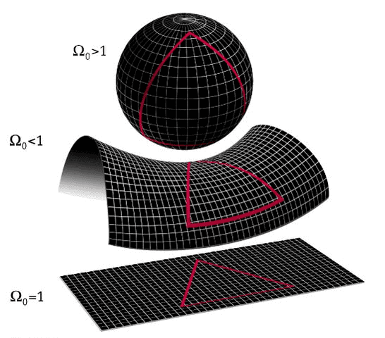
     Fig. 13: The curvature of the universe concerning the current density parameter ^[15]

From the current observations, we can write the values of

$Ω_{mat}, Ω_{rad}$ and $Ω_κ$

$Ω_{mat}=0.0429$ (or you may seem as $Ω_{b}$, $b$ represents the baryonic matter)

$Ω_{rad}≅0$

$Ω_{rad}≅0$

(Planck Mission-2015 results ^[16])

If we put these values in $(4.19)$

$$Ω_{mat}+Ω_{rad}+Ω_κ=0.0429<1~~~~~(4.20)$$

We get a value that is less than $1$. It seems there’s a problem because the sum of the density values must be equal to $1$, which is not.

In the next chapter, we will discuss this problem, and try to understand the missing part. As we will see that, the problem is not that dark.

References

1-Riddle, A. (2003). An introduction to modern cosmology (p. 25).

2-Metric in positively curved two-dimensional space (http://people.virginia.edu/~dmw8f/astr5630/Topic16/Lecture_16.html)

3-Metric (https://en.wikipedia.org/wiki/Metric_(mathematics)) (para.1).

4-Ryden, B. (2006). Introduction to cosmology (pp. 39-49).

5-Cosmological Redshift Picture (http://www.pitt.edu/~jdnorton/teaching/HPS_0410/chapters/big_bang_FRW_spacetimes/)

6- Ryden, B. (2006). Introduction to cosmology (pp. 51-52).

7-Introduction to cosmology (http://www.astronomy.ohio-state.edu/~dhw/A5682/notes4.pdf)

8-Energy density diagram (https://ned.ipac.caltech.edu/level5/Peacock/Peacock3_1.html )

9- Ryden, B. (2006). Introduction to cosmology (p.81).

10- Riddle, A. (2003). An introduction to modern cosmology (p. 23).

11-Density of the universe (https://sites.ualberta.ca/~pogosyan/teaching/ASTRO_122/lect31/lecture31.html)

12-Riddle, A. (2003). An introduction to modern cosmology (p. 39).

13- Cosmological Parameters and Their Evolution (http://www.astronomy.ohio-state.edu/~dhw/A873/p2.pdf)

14- Riddle, A. (2003). An introduction to modern cosmology (p. 47).

15-Flatness Problem (https://en.wikipedia.org/wiki/Flatness_problem)

16- Planck Collaboration. (2015). Planck 2015 results. XIII. Cosmological parameters (p.6) (https://arxiv.org/abs/1502.015899)