Signature of the Sun: Analyzing the Solar Balmer Series Lines

Introduction

We are in many ways a fortunate generation having so many wonderful tools at our disposal on account of the “silicon revolution”. The advent of powerful personal computers has radically changed just about every form of human activity in a few short decades (this author – for example – is of a generation that still used slide rules at school !). Can one imagine – for example – doing linear regression or even simple standard deviation calculations without the use (at very least) of a pocket calculator? In respect of science education, there are many possibilities for effecting realistic computer simulations of any number of experiments that would otherwise demand access to well-equipped laboratories. This is not to run down the necessary ‘ hands-on’ requirements of scientific investigation but rather to consider imaginative ways and means whereby data can be collected and processed in a meaningful scientific manner. Students should be trained to make effective use of spreadsheets and the many excellent built-in statistical routines they contain to process their experimental data. In this article, we will be making use of regression analysis to process data from the ultimate parent of all data generators – our very own sun!

Pixel Ruler Spectroscopy

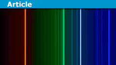
A typical spectrum of whatever element or molecule obtained in the laboratory or from the sun or stars via appropriate optical equipment is essentially a series of lines representing the wavelengths of various electron transitions associated with that element/molecule or set of elements/molecules.  In order to measure the wavelengths from a ‘raw spectrum’, the essential requirements are a ruler and a means whereby a wavelength scale can be established if not already provided.  In this article, we will employ a ‘pixel ruler’ as our measuring device and we will relate pixel measurements to wavelengths through the use of standard lines having known wavelengths. In principle, one needs just two such standard lines in order to establish a pixel/wavelength scale but for more accurate work, one would probably want to use a number of standards and establish the scale through the use of linear regression.  In this article, we will begin with a simple two-line scale. Our data set will be the “Flash Spectrum of the Sun” which arises from photographing the solar chromosphere during an eclipse when – for a brief moment – emission lines, rather than absorption lines, dominate the solar spectrum.

Experimental Objective

Our experimental objective will be to obtain a value of the Rydberg constant (for Hydrogen) by carrying out regression analysis on a set of measurements of Hydrogen’s Balmer series lines. These have wavelengths within the visible range from approximately 350 to 700 nm. Helium spectral lines – also in the visible range – will be used as wavelength standards for calibrating a pixel/Angstrom wavelength scale.

Theory

For Hydrogen’s Balmer series lines, the Rydberg formula is as follows: $$ \frac{1}{\lambda}=R_H\left(\frac{1}{4}-\frac{1}{n^2}\right): n>2 $$ Since we wish to work with wavelengths rather than wavenumber, we need to take reciprocals on both sides obtaining: $$ \lambda = \frac{4}{R_H}\left(\frac{n^2}{n^2-4}\right):n>2$$ Note that if $n→\infty$, the expression simplifies to $\lambda=4/R_H$ which is the wavelength corresponding to the Balmer series limit. Since the expression is of the form y = kx with $y=\lambda$ and $x=\frac{n^2}{n^2-4}$, we can apply regression statistics using measured Balmer series wavelengths against the expression $\frac{n^2}{n^2-4}$ to obtain a value of the constant k and hence determine an empirical value for $R_H$ the Rydberg constant for Hydrogen. Values of n for Balmer series lines in the visible spectrum are from 3 to 6.

An experimental subtlety that should be noted is that the theory applies specifically to wavelengths ‘in vacuo’ whereas the (visible) solar spectrum we will be using as our data set is typically derived from photographs taken in an air medium. Conversion of wavelengths from air to vacuum is somewhat complicated but for our purposes, it will be sufficient to use the factor 1.0003 corresponding to the air/vacuum refractive index.

Method

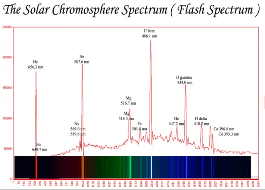
Appendix A below is a solar “flash spectrum” taken during an eclipse of the sun. Most of the spectral lines are already marked with wavelengths but since our purpose is to measure, we will largely ignore these or simply use them as checks for the data obtained. We will be using a pixel ruler to measure (in pixels) the position of the four Hydrogen Balmer series lines as well as two Helium lines to be used for calibration purposes. The relevant Helium lines are the bright yellow line at 5875.6148 Å and the weaker peak at 4471.479 Å (air wavelengths). Note that since these will be used for calibration purposes, we should not have any experimental ‘qualms’ about using all the decimal digits available (the wavelengths are taken from NIST’s spectral database).

Next, the 4 Balmer series lines will be measured in pixels and converted to measured wavelengths using the calibration equation from the Helium lines. Finally, the regression analysis described above will be carried out and the Rydberg constant $R_H$ calculated from the value of “k” the gradient of the regression line.

Calibration

The graphic below shows a measurement of the Helium yellow line at 428 pixels from the left edge of the screen.

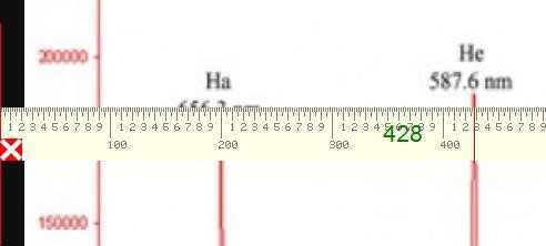
Similarly the measurement for the second Helium line is at 894 pixels and so our simple linear calibration curve will be of the  form y = mx + c with (y) being the measured wavelength determined from the pixel measurement (x).$$ m = \frac{4471.479 – 5875.6148}{894 – 428} $$ and: $$ c = 5875.6148 – \frac{4471.479 – 5875.6148}{894 – 428}\times 428 $$

Table of Results and Calculations

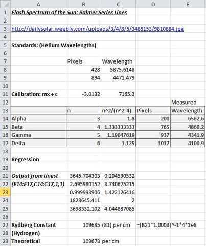
The snapshot of an Excel spreadsheet below shows the processing of the measurements obtained above. The Helium lines are used to obtain a calibration equation which is then used to convert the pixel measurements of Balmer series lines into wavelengths. Regression of column E against column C yields the Balmer series limit (B21) from which the Rydberg constant (for Hydrogen) can be calculated (B27). Note the relevant calculation (and correction for air/vacuum) shown in D27 below.

Discussion of Results and Conclusion

The above ‘experiment’ required minimal equipment other than a PC with Internet access and some form of pixel ruler software loaded. All the same, it yielded a result differing from the well-established theoretical value (of the Rydberg constant for Hydrogen) by just 64 ppm. Albeit dwarfed somewhat by the measurement’s error margin of  +- 740 ppm which arises from the uncertainty (B22 above) in the value of the Balmer series limit value (B21) . Another very encouraging aspect of the results obtained was that the calibrated wavelengths of Balmer series lines were in good agreement with their established values and that there was an excellent correlation (B23 above) of wavelengths against the Balmer series number pattern n^2/(n^2 – 4).

Theoretically, the regression line should go through the origin but the y-intercept obtained (C21 above)  is very small and also dwarfed by the associated error margin of nearly 4 Å.  One could “force through zero” using options available in the Excel “linest” function but otherwise, just accept that the small offset obtained is an expected artefact of the statistical process.

From an educational perspective, this ‘practical’ would hopefully provide students with an opportunity to learn about some of the most prominent lines in the solar spectrum and to understand the Rydberg equation particularly as it applies to the Balmer series members in the visible spectrum. It should also encourage careful measurement along with the use of calibration curves and of regression analysis as well as the skill of determining appropriate measurement error margins.

 

Appendix A: The Flash Spectrum of the Sun

Image Credit: http://dailysolar.weebly.com/uploads/3/4/8/5/3485153/9810884.jpg

Appendix B: Spectrum of the Chromosphere: S.A Mitchell, January 1930

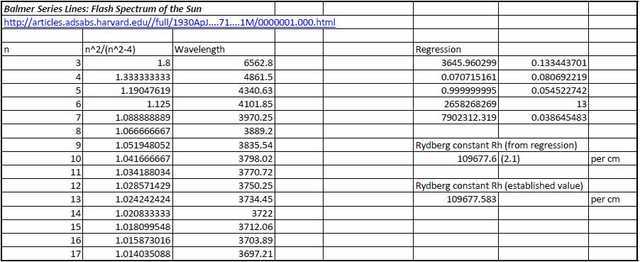
By way of comparison with the fairly ‘rough and ready’ data set obtained above, the following is a data set and included regression analysis carried out on wavelengths of Balmer Series lines up to n=17 obtained from solar eclipses in 1905 and 1925. We will leave the author to describe the means whereby his spectrum was obtained:

“The spectra of the 1905 eclipse were secured in Spain while I was a member of the United States Naval Observatory Expedition. The photographs of the flash spectrum were obtained by two different grating spectrographs, each used without slit. One of the gratings was concave, of 10-foot radius, ruled with 14,438 lines per inch, the so-called “parabolic” grating of 4-inch aperture. The other was a plane grating of 15,000 lines per inch and 6-inch aperture. The discussion of the spectra is found in the Astrophysical Journal, 38, 407, 1913, in Publications of the Leander McCormick Observatory, 2, Part 2, and also in Publications of the U.S. Naval Observatory, 10, B, 32-116,1924.”

From: Spectrum of the Chromosphere

We will further leave the regression statistics to speak for themselves!

Acknowledgments

Many thanks to PF member Dr. Courtney for reviewing this article and suggesting greater clarity on error margins as well as prompting the note concerning the y-intercept of the regression analysis.

References

 

[1]	A. Kramida, Yu. Ralchenko, J. Reader, and and NIST ASD Team. NIST Atomic Spectra Database (ver. 5.6.1), [Online]. Available: https://physics.nist.gov/asd [2019, September 4]. National Institute of Standards and Technology, Gaithersburg, MD., 2018. [ bib ]
[2]	Elizabeth Observatory of Athens. Flash spectrum of the sun, 2015. [ bib | http ]
[3]	S. A. Mitchell. The Spectrum of the Chromosphere. , 71:1, Jan 1930. [ bib | DOI ]

 

Comment Thread