
Learn Statistical Mechanics: Equilibrium Systems
This is the first of a multi-part series of articles intended to give a concise overview of statistical mechanics and some of its applications. These articles are by no means comprehensive of the entire field but aim to give a clear line of reasoning from Boltzmann’s equation to non-equilibrium statistical mechanics. It is hoped that these articles will help the reader to better understand the framework of statistical mechanics as well as the concepts of entropy and the second law, which are notoriously slippery concepts to fully grasp, even for practicing physicists.
Statistical mechanics aims to predict the macroscopic behavior of many-body systems by studying the configurations and interactions of the individual bodies. Statistical mechanics is often taught as an extension of thermodynamics. This is helpful since it can give a clearer understanding of thermodynamic quantities such as temperature and entropy. However, the application of statistical mechanics is not constrained only to thermodynamic problems. Indeed, it has been successfully applied to many problems outside of pure physics: a few examples include the behavior of stock markets, the spread of disease, information processing in neural nets, and self-segregation in neighborhoods.
Table of Contents
Gibbs Entropy and the Boltzmann Equation
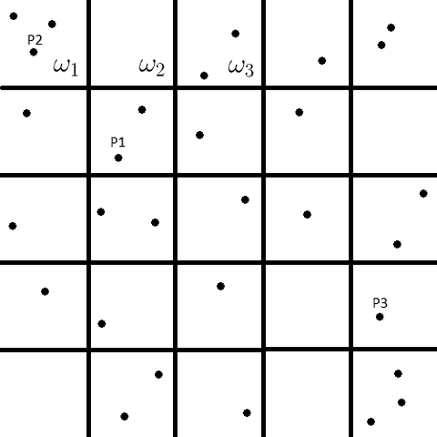
To begin, consider a collection of subsystems simultaneously occupying the phase space ##\Omega_{E}## where ##\Omega_{E}## is a subspace with constant energy ##E## of the total phase space. The nature of the subsystems is left unspecified for the sake of generality. Now consider that the positions and momenta are discretized such that ##\Omega_{E}## is partitioned into ##l## discrete cells labeled ##\omega_{1},\omega_{2},\cdots\omega_{l}## as shown below. Each point ##P_{i}## represents the particular state of a subsystem in phase space.
Let ##\omega_{i}## represent the number of sub-systems consistent with the ##i##th thermodynamic state. The number of subsystems in all the accessible states must sum to the total number of subsystems as
$$\sum_{i=1}^{l}\omega_{i}=\Omega_{E}$$
The distribution ##D=\{\omega_{1},\omega_{2},\cdots\omega_{l}\}## describes the state of the whole system. The number of arrangements ##W(D)## consistent with a given distribution is
$$W(D)=\frac{\Omega_{E}!}{\omega_{1}!\omega_{2}!\cdots\omega_{l}!}$$
The claim crucial to the formulation of statistical mechanics is that the entropy ##S## of a system and the quantity ##W## are related. Low entropy states correspond to small ##W## while high entropy states correspond to large ##W##. Thus, high entropy states are much more numerous than low entropy states. Since the particle dynamics are considered stochastic, states are selected at random. This naturally leads to a preference for high entropy states over low entropy states. In the thermodynamic limit (as ##N## and ##V## goes to infinity with ##\rho## constant), the number of high entropy states grows continuously larger than the number of low entropy states. This forces the system to exist in the maximum entropy state when at equilibrium.
The function that maps ##W## to ##S## must meet certain criteria for ##S##.
- ##S## is a continuous function of ##W##
- ##S## is a monotonically increasing function of ##W##: If ##W_{1}>W_{2}## then ##S(W_{1})>S(W_{2})##
- ##S## is additive: ##S(W_{1}W_{2})=S(W_{1})+S(W_{2})##
The first two criteria follow from the above arguments to express ##S## in terms of ##W##. The third criterion is required to make the entropy an extensive quantity. When two separate subsystems are combined, the number of arrangements of the combined system is the product of the number of arrangements of each subsystem and the entropy of the combined system is the sum of the entropy of each subsystem.
The simplest function satisfying these criteria, as postulated by Boltzmann, is proportional to a logarithmic function.
$$S=k\ln W=k\ln \frac{\Omega_{E}!}{\omega_{1}!\omega_{2}!\cdots\omega_{l}!}$$
Using Sterling’s approximation, this can be written as
$$S=k\left[\Omega_{E}\ln \Omega_{E} -\Omega_{E} -\sum_{i=1}^{l}\omega_{i}\ln \omega_{i}+\sum_{i=1}^{l} \omega_{i}\right]$$
Defining ##p_{i}=omega_{i}/Omega_{E}## as the probability of finding a subsystem in a particular state ##omega_{i}##, and remembering that ##sum_{i=1}^{l}p_{i}=1##, gives the Gibbs entropy formula
$$S=-k\sum_{i=1}^{l}p_{i}\ln p_{i}$$
Notice that ##S## takes on a minimum value for the delta function distribution ##p_{i}=delta_{i,j}## and a maximum value for the uniform distribution ##p_{i}=1/l##. Thus ##S## is a measure of the dispersity of the distribution ##p_{i}##. I am reluctant to use the term disorder here since such wording is a source of much confusion. A system that looks disordered is not necessarily a high entropy state: examples include the crystallization of supersaturated solutions and liquid crystals. Disorder is furthermore a qualitative term and thus subject to the opinion of the observer.
The maximum entropy probability distribution has special importance here. When a system is initially in a non-equilibrium state, it will evolve in time until it reaches an equilibrium state (assuming one exists), where it will remain forever. The second law of thermodynamics states that the entropy of a closed system tends to a maximum. Thus, the equilibrium state is also a maximum entropy state.
Consider an isolated system with ##\Omega## accessible configurations. At equilibrium, the probability of being in a given state is expected to be constant in time. The system may fluctuate between different microstates but these microstates must be consistent with fixed macroscopic variables, i.e. pressure, volume, energy, etc. There is nothing that would lead us to believe that one microstate is favored over another. Thus we invoke the principle of equal a priori probabilities such that ##p_{i}=1/\Omega##, which is the special case of a uniform probability distribution. This gives the Boltzmann entropy formula:
$$S=-k\sum_{i=1}^{\Omega}\frac{1}{\Omega}\ln\frac{1}{\Omega}=k\ln \Omega$$
The Boltzmann formula is therefore consistent with the maximum entropy state and is a valid description of the entropy of a system at thermodynamic equilibrium.
The Canonical Ensemble
To describe the equilibrium state using the Canonical ensemble (##N##, ##V##, & ##T## constant), we search for the distribution ##p_{i}## which maximizes the Gibbs entropy under the constraints that the probabilities are normalized
$$\sum_{i}p_{i}=1$$
and the average energy is fixed
$$\left<E\right>=\sum_{i}p_{i}E_{i}=U$$
The probability distribution which maximizes the entropy is found using the method of Lagrange multipliers.
$$\mathcal{L}=\left(-k\sum_{i}p_{i}\ln p_{i}\right)+\lambda_{1}\left(\sum_{i}p_{i}-1\right)+\lambda_{2}\left(\sum_{i}p_{i}E_{i}-U\right)$$
$$0=\frac{\partial\mathcal{L}}{\partial p_{j}}=-k-k\ln p_{j}+\lambda_{1}+\lambda_{2}E_{j}$$
$$p_{j}=\exp\left(\frac{-k+\lambda_{1}+\lambda_{2}E_{j}}{k}\right)$$
##\lambda_{1}## is determined by the normalization condition on ##p_{j}##:
$$1=\sum_{j}p_{j}=\exp\left(\frac{-k+\lambda_{1}}{k}\right)\sum_{j}\exp\left(\frac{\lambda_{2}E_{j}}{k}\right)=\exp\left(\frac{-k+\lambda_{1}}{k}\right)Z$$
where ##Z## is defined as
$$Z=\sum_{j}\exp\left(\frac{\lambda_{2}E_{j}}{k}\right)$$
This sets ##\lambda_{1}## as
$$\exp\left(\frac{-k+\lambda_{1}}{k}\right)=\frac{1}{Z}$$
while the probability distribution becomes
$$p_{j}=\frac{1}{Z}\exp\left(\frac{\lambda_{2}E_{j}}{k}\right)$$
To determine ##\lambda_{2}##, we first rewrite ##S## in terms of ##Z## as
$$S=-k\sum_{j}p_{j}\ln p_{j}=-k\sum_{j}p_{j}\left(\frac{\lambda_{2}E_{j}}{k}-\ln Z\right)=-\lambda_{2}U+k\ln Z$$
and use the thermodynamic definition of temperature to find
$$\frac{1}{T}\equiv\frac{\partial S}{\partial U}=-\lambda_{2}$$
The canonical partition function ##Z## is thus
$$Z\equiv\sum_{i}\exp\left(-\beta E_{i}\right)$$
where ##\beta\equiv 1/kT##. The probability distribution and the entropy at equilibrium are
$$p_{i}=\frac{1}{Z}\exp\left(-\beta E_{i}\right)$$
$$S=\frac{U}{T}+k\ln Z$$
The Partition Function and Thermodynamic Variables
With the above definition of the partition function and probability distribution, the relationships between ##Z## and other thermodynamic quantities can now be found. The average energy is
$$\left<E\right>=\sum_{i}p_{i}E_{i}=\frac{1}{Z}\sum_{i}\exp\left(-\beta E_{i}\right)E_{i}=-\frac{1}{Z}\frac{\partial Z}{\partial\beta}=-\frac{\partial}{\partial\beta}\ln Z$$
The heat capacity is
$$C_{v}=\frac{\partial\left<E\right>}{\partial T}=-k\beta^{2}\frac{\partial\left<E\right>}{\partial\beta}=k\beta^{2}\frac{\partial^{2}}{\partial\beta^{2}}\ln Z$$
The Helmholtz free energy is
$$F=U-TS=-kT\ln Z$$
which gives a more direct representation of the entropy as
$$S=-\frac{\partial F}{\partial T}=k\frac{\partial}{\partial T}T\ln Z$$
Many macroscopic quantities of interest can be found if the partition function is known. It is often said that if the partition function is known, then everything is known about the system. Thus the goal when studying the behavior of equilibrium systems is to find the partition function ##Z##, from which all other useful information can be obtained.
Education: Graduate student in physics; specializing in biophysics and non-linear dynamics.
Hobbies: Astrophotography, Electronics, and Mineral collecting


In part 1 in the paper on 4/9 : S = k ln W = k ln Ω[SUB]E[/SUB] ! /ω[SUB]1[/SUB] !ω[SUB]2[/SUB] !…ω[SUB]l[/SUB] !
And on page 5/9 : S = k ∑[SUB]i =1[/SUB][SUP]Ω[/SUP] 1/Ω ln 1/Ω = k ln Ω
In part 2 first paragraph Ω[SUB]E[/SUB] = (N+v-1)! / N!(v-1)!
In what physical situations does S = k ln W apply ?
And in what physical situations does S = k ln Ω apply ?
From my text ( Halliday Resnick ) W is defined (V)[SUP]N[/SUP] And they say that S = k ln W for entropy state for non equilibrium systems ? Is there a basic corresponding definition for Ω ?
What are the qualitative / quantitative differences between W and Ω
I undestand I am asking a B level question in an advanced topic
Thank you
Part 2 is up
https://www.physicsforums.com/threads/statistical-mechanics-part-ii-the-ideal-gas-comments.942669/
I don't know, where this inaccurate information comes from. I guess, what's meant is the path-integral formulation of quantum field theory. In QFT the "sum over paths" is in fact a functional integral (which is hard to properly define; to my knowledge it's not mathematically rigorously defined today) over field configurations.
The path integral comes in many forms. Two are most important:
(a) in vacuum QFT, which deals with scattering processes of a few particles, that can be depicted as the usual Feynman diagrams for the evaluation of S-matrix elements in perturbation theory. The Feynman diagrams depict formulae for S-matrix elements evaluated in perturbation theory. A diagram with ##n## external points depicts the time-ordered ##n##-point Green's functions of the theory. The same quantity can also be derived from a generating functional, which is given in terms of a path integral as
$$Z[J]=int mathrm{D} phi int mathrm{D} Pi exp[mathrm{i} S[phi,Pi]+mathrm{i} int mathrm{d}^4 x J(x) phi(x)],$$
where
$$S=int mathrm{d}^4 x [phi(x) Pi(x) – mathcal{H}(Phi,Pi)]$$
is the action in terms of its Hamiltonian formulation, ##phi## is a set of fields and ##Pi## their canonical field momenta.
Unfortunately you can evaluate only path integrals where the action is a bilinear form of the fields and canonical field momenta, i.e., a Gaussian functional integral. This refers to free fields. So you split the action in the bilinear free part and the higher-order interaction part and expand the Path integral in terms of powers of the interaction part. What you get is a formal power series of the corresponding coupling constants and yields the same result as time-dependent perturbation theory when using the more conventional operator formalism ("canonical field quantization").
From this it beomes clear that what you evaluate in fact is the time evolution of the theory with a time-evolution operator
$$hat{U}(t,t')=exp(-mathrm{i} int_{t'}^t mathrm{d} tau int mathrm{d}^3 vec{x} mathcal{H}.$$
Usually after some care using "adiabatic switching" you make ##t' rightarrow -infty## and ##t rightarrow +infty## to finally obtain the LSZ-reduction formalism to evaluate the S-matrix elements from the corresponding ##n##-point timeordered Green's functions.
(b) in equilibrium many-body theory you usually are after the canonical or grand-canonical partition function, which is in the operator formalism given by
$$Z=mathrm{Tr} exp(-beta hat{H}),$$
where ##beta=1/k_{text{B}} T## is the inverse temperature (modulo the Boltzman constant, which we set to 1 in the following). The expression under the trace now looks like a time-evolution operator with the time running along the imaginary axis from ##0## to ##-mathrm{i} beta##, and that's used in the path-integral formalism: Thus as you can express the generating functional for time-ordered Green's functions as a path integral over field configurations you can evaluate the partition sum as a path-integral with an imaginary time.
Making the time imaginary leads to an action in Euclidean QFT, i.e., instead of the usual Minkowski-space action you get an action as if spacetime where a four-dimensional Euclidean space. Taking the trace leads to periodic (for bosons) or antiperiodic (for fermions) boundary conditions in imaginary time, i.e., the fields over which to integrate are subject to the constraint ##phi(t-mathrm{i} beta,vec{x})=pm phi(t,vec{x})## with the upper (lower) sign for bosons (fermions), the socalled Kubo-Martin-Schwinger (or short KMS) conditions.
With that mathematical trick you get the same Feynman rules to evaluate the partition sum in this imaginary-time (or Matsubara) formulation of many-body QFT as in vacuum QFT with the only difference that internal lines stand for the Matsubara propagator, and instead of energy integrals in the energy-momentum version of the Feynman rules you have to sum over the Matsubara freqencies ##mathrm{i} 2 pi T n## (bosons) or ##mathrm{i} pi T (2n+1)## with ##n in mathbb{Z}##.
I am having a hard time understanding why phase state represents the particle / system path through time and the connection of it with thermodynamic states. Where can I find more info about it? I have been reading Marion's Classical Dynamics, but it did not help. tks
What software are you using?Windows 10 with Google Chrome Version 64.0.3282.167
I'm having trouble with the Latex rendition of this Insights articleWhat software are you using?
One of my computers has an old version of Firefox 38.0.5 and it can have weird errors in displaying pages.
For example, @Philip Koeck 's researchgate article at https://www.researchgate.net/public…_distribution_for_indistinguishable_particles is displayed with a wierd error that omits some letter combinations like "ti".
View attachment 221017
That's strange, do you have any idea what could be causing this? It looks normal on my computer.
I'm having trouble with the Latex rendition of this Insights article. It seems that many of the symbols appear doubled. Below is a screen shot of what I'm seeing.
View attachment 221009
Does the phrase "with constant energy" mean that each microstate in ΩEΩEOmega_E has the same energy EEE?Yes, here I am working with the microcanonical ensemble where ##E## is fixed. Perhaps I should clarify this.
I don't understand how the "EEE" in this section is related to the "EEE" in the first paragraph of the article. Is "EEE" is being used both to denote a constant and a random variable?This part is from the canonical ensemble where the temperature is fixed rather than the energy being fixed. The first section assumes constant energy and the second section assumes constant temperature.
How is EiEiE_i defined ?##E_{i}## is the energy of the ##i##th state.
Which books did you read?Its too long ago to remember titles. The first text I see on my bookshelf is Statistical Physics by F. Mandl, but I didn't read much of that book.
—-
##Omega_E## is a subspace with constant energy ##E## of the total phase space.Does the phrase "with constant energy" mean that each microstate in ##Omega_E## has the same energy ##E##?
##<E> =sum_i p_i E_i = U##I don't understand how the "##E##" in this section is related to the "##E##" in the first paragraph of the article. Is "##E##" is being used both to denote a constant and a random variable?
How is ##E_i ## defined ?
Are we assuming that any "bias" in the finite set of subsystems is supposed to be overcome by the fact we attain a representatives sample as the number of subsystems under consideration approaches infinity?I never actually gave a value for any of the probabilities; I only assumed that they exist. As far as a real system is concerned, equilibrium statistical mechanics generally requires something approaching the thermodynamic limit to give a reasonable answer.
Suppose Bob partitions ΩEΩEOmega_E into 10 states b1,b2,…b10b1,b2,…b10b_1,b_2,…b_{10} and Alice partitions ΩEΩEOmega_E into 10 states a1,a2,…a10a1,a2,…a10a_1,a_2,…a_{10} in a different manner. Setting pb1=ωb1/ΩE=1/10pb1=ωb1/ΩE=1/10p_{b_1} = omega_{b_1}/Omega_E = 1/10 might give a different model for a random measurement than setting pa1=ωa1/ΩE=1/10pa1=ωa1/ΩE=1/10 p_{a_1} = omega_{a_1}/Omega_E = 1/10. For example, Alice might have chosen to make her a1a1a_1 a proper subset of Bob's b1b1b_1.The way that the phase space is partitioned is not completely arbitrary. Each ##omega## must only enclose identical states.
You mentioned that you have read other introductory books on statistical mechanics but did not find the exposition clear. Which books did you read? I would recommend both Statistical Physics of Particles and Statistical Physics of Fields by Mehran Kardar. The first book builds up the theory in a manner similar to what I have done here but with more background information.
I realize the Insight is intended as an overview of Statistical mechanics as oppose to an introduction to it. However, I'll comment on the logic structure since I've never found an introduction where it is presented clearly -and perhaps someday you'll write a textbook.
My point was that since the subsystems are identical, if you relabel the points, one could not tell which points have been relabeled or which points have been moved. This allows for the a priori probability distribution ##p_{i}=omega_{i}/Omega_E##.I don't see that the subsystems are "identical".
My interpretation: Apparently the underlying probability space we are talking has outcomes of "pick a subsystem". If we assume each subsystem has an equal probability of being selected, then it follows that the probability of the event "we select a subsystem in state ##i##" is ##omega_i/Omega##.
The conceptual difficulty in applying this to a particular physical system (e.g gases) is that we are dealing with a finite set of points in phase space and nothing is said about how these points are selected. If the goal is to model what happens in experiments, the we should imitate how an experiment randomly encounters a subsystem. For example, if we are modeling the event "A randomly selected person's last name begins with 'X"" by randomly selecting a person from a set of people then we need a set of people whose last names are representative of the entire population.
Are we assuming that any "bias" in the finite set of subsystems is supposed to be overcome by the fact we attain a representatives sample as the number of subsystems under consideration approaches infinity? For a finite population, we would achieve a representative sample that was the whole population. However, I don't see why taking more and more points in a (continuous) phase space necessarily guarantees a representative sample.
I defined equilibrium as a maximum entropy state.Did you define equilibrium?
You wrote:
At equilibrium, the probability to be in a given state is expected to be constant in time.Do we take that as the definition of equilibrium?
Justifying that the maximum entropy distribution gives the probabilities that would occur in a random measurement of a system at equilibrium seems to require an argument involving the limiting probabilities of a random process .
The system may fluctuate between different microstates but these microstates must be consistent with a fixed macroscopic variables, i.e. pressure, volume, energy, etc. There is nothing which would lead us to believe that one microstate is favored over another.Suppose Bob partitions ##Omega_E## into 10 states ##b_1,b_2,…b_{10}## and Alice partitions ##Omega_E## into 10 states ##a_1,a_2,…a_{10}## in a different manner. Setting ##p_{b_1} = omega_{b_1}/Omega_E = 1/10 ## might give a different model for a random measurement than setting ## p_{a_1} = omega_{a_1}/Omega_E = 1/10##. For example, Alice might have chosen to make her ##a_1## a proper subset of Bob's ##b_1##.
So something about the condition "these microstates must be consistent with a fixed macroscopic variables" needs to be invoked to prevent ambiguity. I don't see how this is done.
—–
Using Sterling’s approximation, this can be written as S=k[ΩElnΩE−ΩE−∑i=1lωilnωi+∑i=1lωi]It's worth reminding readers that the error in Sterling's approximation for ##N!## approches infinity as ##N## approaches infinity. So finding the limit of a function of factorials cannot, in general, be done by replacing each factorial by a Sterling's approximation. For the specific case of multinomial coefficients, the replacement works. ( If we encounter a situation where we are letting the number of factorials in the denominator of a binomial coefficient approach infinity, I'm not sure what happens. For example, if we need to take a limit as we partition ##Omega_E## into more and more ##omega_i##, it might take some fancy analysis.)
Does that assumption have a physical interpretation?My point was that since the subsystems are identical, if you relabel the points, one could not tell which points have been relabeled or which points have been moved. This allows for the a priori probability distribution ##p_{i}=omega_{i}/Omega##.
it seems to me that we are effectively defining "equilibrium" to mean that the probability of sss being in state iii is constant with respect to time.I defined equilibrium as a maximum entropy state. There is nothing preventing the probabilities from having some sort of time dependence. The Gibbs entropy is technically valid even in non-equilibrium systems.
##omega## represents an accessible state in the phase space so when ##omega## is used to denote the number of subsystems in the cell it is denoting the number of subsystems occupying a given state in the phase space.That may be traditional notation in physics. However, it would more precise to use the subscript ##i## as the "label" for the "state" (or "cell") and notation ##omega_i## the symbol for the number of subsystems in state ##i##. If there needs to be a discussion about the spatial volume of a state ##i## in phase space, that volume would require yet another symbol.
The assumption is that since each subsystem is identical, each can arbitrarily switch positions with another subsystem. This leads to the distribution ##p_{i}=omega_{i}/Omega_{E}##.Does that assumption have a physical interpretation? Or is "switch positions" just a mental operation that we can do by re-labeling things?
Presumably we seek to model an experiment where a system is prepared to have total energy ##E## and is at "equilibrium". We model this by picking a subsystem ##s## at random from the set of subsystems giving each subsystem the same probability of being selected. If we make an ergodic hypothesis that the probability of ##s## being in state ##i## remains constant in time then there is a probability of ##omega_i/Omega_E## that the system ##s## is in state ##i##. Since your exposition hasn't yet dealt with gases or other processes where "equilibrium" has a technical definition, it seems to me that we are effectively defining "equilibrium" to mean that the probability of ##s## being in state ##i## is constant with respect to time.
Of course, I have similar complaints about all other expositions of statistical mechanics that I have read. They seem to invite the reader to make the elementary mistake of assuming that if there are N possibilities then each possibility must necessarily have probability 1/N. (e.g. There are 26 letters in the alphabet, so the probability that a randomly chosen citizen has a last name beginning with "X" is 1/26.)This is not what is being assumed though. Using this example, each ##omega## would represent a letter of the alphabet. Since more people have a last name starting with S then X, there will be many more points in ##omega_{S}## then ##omega_{X}##. The probability of someone's last name beginning with X would be ##p_{X}=omega_{X}/Omega## where ##Omega## is the total number of people.
Notice however that if the probability of each letter was equal, then this would be a maximum entropy state where ##p_{i}=1/26## and the entropy would follow the Boltzmann equation.
What you call "microcanonical" is usually called "canonical".Thanks for pointing that out. I will correct that.
The "ωiωiomega_i" is introduced as a notation for a "cell" in phase space, but then ωiωiomega_i is used again to denote the number of subsystems in a cell. It this ambiguous notation ? – or is there some distinction made in the typograhy that I'm not recognizing?##omega## represents an accessible state in the phase space so when ##omega## is used to denote the number of subsystems in the cell it is denoting the number of subsystems occupying a given state in the phase space.
The choice of the word "Defining" is interesting. Can we arbitrarily define the probability of finding a "random" subsystem in a particular state ωiωiomega_i?
It seems to me that such a definition involves some implicit assumption about the way the phase space has been divided into cells. For example, if the distribution of subsystems in phase space is uniform over its volume and we use cells that all have the same volume, we could deduce that the probability of finding a subsystem chosen from this uniform distribution to be in cell ωiωiomega_i is the ratio of the volumes ωi/ΩEωi/ΩEomega_i/ Omega_E.The size of ##omega## is arbitrary. The definition of the probability ##p_{i}## is made by counting the number of subsystems which can occupy the section of phase space ##omega_{i}##. The assumption is that since each subsystem is identical, each can arbitrarily switch positions with another subsystem. This leads to the distribution ##p_{i}=omega_{i}/Omega_{E}##.
What you call "microcanonical" is usually called "canonical". In the microcanonical ensemble the energy is strictly in a little shell around a fixed value ##E_0##. It's for a closed system. In the microcanonical ensemble the energy is fixed only on average, i.e., you have an open system, where energy exchange with the environment or a heat bath is possible, but no particle exchange. Finally, the grand-canonical ensemble is the case, where the open system can exchange both energy and particles with the environment.
Defining pi=ωi/ΩE as the probability to find a subsystem in a particular state ωi,The choice of the word "Defining" is interesting. Can we arbitrarily define the probability of finding a "random" subsystem in a particular state ##omega_i##?
It seems to me that such a definition involves some implicit assumption about the way the phase space has been divided into cells. For example, if the distribution of subsystems in phase space is uniform over its volume and we use cells that all have the same volume, we could deduce that the probability of finding a subsystem chosen from this uniform distribution to be in cell ##omega_i## is the ratio of the volumes ##omega_i/ Omega_E##.
Alternatively, we could have a non-uniform distribution of substems over the phase space and explicitly say that we choose the division into cells in such a manner that the probability that a system chosen from this distribution being in a particular cell is the ratio of the volume of the cell to the total volume of the phase space.
Of course, I have similar complaints about all other expositions of statistical mechanics that I have read. They seem to invite the reader to make the elementary mistake of assuming that if there are N possibilities then each possibility must necessarily have probability 1/N. (e.g. There are 26 letters in the alphabet, so the probability that a randomly chosen citizen has a last name beginning with "X" is 1/26.)
The "##omega_i##" is introduced as a notation for a "cell" in phase space, but then ##omega_i## is used again to denote the number of subsystems in a cell. It this ambiguous notation ? – or is there some distinction made in the typograhy that I'm not recognizing?