What Thermodynamics and Entropy Means

Introduction

The student of thermodynamics, as they consider pistons and ideal gasses and such, often begin to grasp the nature of entropy only to find as they delve deeper that grasp slips away.  In the deeper analysis of thermodynamic systems via statistical mechanics this grasp may slip away entirely.

“How can my cup of hot tea, have a given entropy from instant to the instant when at any given instant it is in some exact physical state whether I know which one it is or not?” “If entropy is a measure of disorder then what makes one state more ordered than another?  By what divine aesthetic is order measured?”

One begins to think entropy is merely an on-paper quantity describing only an aspect the probability distributions of various states of reality.  But, when a sip of that hot tea burns the tongue the immediately physical nature of entropy becomes very hard to deny.

Thermodynamics and Entropy

Joule’s Demonstration

James Joule discovered the mechanical equivalent of heat in a classic demonstration where a falling weight is used to stir an insulated container of water causing its temperature to rise.

This pointed to the possibility of the reverse process, producing mechanical work from heat.

Sadi Carnot, a 19th-century French physicist coined the term entropy in his study of steam engines.  Later Rudolf Clausius was able to quantify the extent to which energetic processes were recoverable and how much heat energy could be recovered as useful work.

Clausius’ formula below expresses how this quantity, entropy, changes when a body absorbs or emits heat energy.

$$\delta S = \frac{\delta Q}{T}$$

Somehow within the internal workings of material systems entropy relates to heat energy and temperature.

How Entropy Is Used, The Carnot Cycle

Consider a piston containing a gas.  We can increase or decrease its temperature in two distinct ways.  If, while keeping the piston insulated from it surroundings, we compress the gas or allow it to expand its temperature will go up or down as will its pressure.  Alternatively, we can place the piston in contact with a higher or lower temperature object, say a hot plate or ice bath and let the heat flow into or out of the gas.

Now suppose we heat the gas to a higher temperature by one of these means and then lower it back to its original temperature.  With an insulated piston, it takes mechanical work to compress it and we can recover that work as it expands.  The gas is acting just like a spring.  There is no change of entropy, the process is isentropic.

If however, we place the piston in contact with a heat reservoir (hot plate) to bring the temperature up and then a heat dump (ice bath) to cool it down.  Then there was a net flow of heat from the heat reservoir to the heat dump.  The final configuration when we consider these as well as the piston has changed.  There has been a net change of entropy.

We can also combine the two processes.  Start with the piston at the same temperature $T_1$ as the heat reservoir and allow it to expand doing work but slowly enough that the temperature remains constant.  This is \emph{isothermal} expansion.  In practice, this will be infinitely slow.  To speed it up the gas in the expanding piston would be slightly cooler than the heat source so that heat will flow into it.  But in this idealized limit, the Clausius formula tells us how much the entropy of the piston has increased,
$$\Delta S = \frac{Q_1}{T_1}$$
where $Q_1$ is the amount of heat energy that flowed out of the heat source.

Now we detach the piston from the heat source and we want to do the same in reverse for the heat sink so we let the piston undergo isentropic expansion doing more work until it cools to the temperature of our heat sink, $T_2$.  We let $W_1$ represent the total work done in these two stages.

Now we connect the piston to the heat sink and compress it slowly keeping the temperature very close to $T_2$.  Our goal is to dump the entropy gained earlier so that the piston can later be brought back to its initial state.  This means we compress it until the amount of heat $Q_2$ has exited the piston into the heat sink where,

$$\Delta S = \frac{Q_2}{T_2}$$

This will take some work.  We also will need to perform another isentropic compression which will require some work to get the gas back up to the temperature $T_1$ for the start of the cycle, call the work required for both these steps $W_2$ and let $\Delta W = W_1 – W_2$ be the net amount of work taken out of the piston for the full cycle.

This is the classic Carnot cycle and tells us the maximum amount of work we can get out of a heat engine.  Conservation of energy tells us that $\Delta W=Q_1 – Q_2$.  The net-zero change in the entropy of the gas tells us that,

$$\frac{Q_1}{T_1}=\frac{Q_2}{T_2}, \text{ or } Q_2 = Q_1\frac{T_2}{T_1}$$

The thermodynamic efficiency of the cycle is the proportion of heat converted to work:

$$\eta=\frac{\Delta W}{Q_1}=\frac{Q_1 – Q_2}{Q_1}= 1-\frac{T_2}{T_1}$$

Notice that to achieve 100% efficiency is to have a heat sink at absolute zero.  (These temperatures are in absolute units i.e. Kelvin or Rankine.)

So from exploring the Carnot cycle and how Clausius’ formula is applied we see entropy tells us something about the transfer of energy in the form of heat.  Consider now one more step in this cycle.  Suppose that after recovering all of that lovely useful work, we use it to merely generate more heat which we dump into the heat sink.  We might as well have brought the heat source and sink into contact with each other and let the heat flow directly.  But considering it in these terms we can see how the process of converting mechanical work to heat at a given temperature as demonstrated by Joule leads to an increase in the entropy associated with that energy.

Entropy as a Measure of Ambiguity

Entropy has often been described as a measure of disorder.  However, in my “disorderly” house, I remember where most everything is.  While it is a mess I can quickly identify what stack something is in, and guess fairly accurately how deep it is in the stack based on how long it’s been since I last saw it.  However, when I had a housekeeper coming in to clean twice I week, I was hard-pressed to find anything after she had put my house “in order”.  While I would often, tongue-in-cheek list entropy reversal in the ‘for’ line of my checks to my housekeeper I was in point of fact misrepresenting the meaning of entropy.

So let us consider a much simpler example than the disarray of my home.  Consider the situation where I have six blocks, three of which are red and three of which are green.  Now consider two arrangements:

Arrangement 1

 

Arrangement 2

One might use these as examples of a system with lower entropy (Arrangement 1) vs higher entropy (Arrangement 2).  However, technically both situations have zero entropy because there is no ambiguity in the arrangements (at the level at which we are considering it).  To see that the ‘order’ vs ‘disorder’ quality is relative consider now a distinct way of labeling the blocks.

If I label each block with the following sequences of 10 X’s and O’s.  You’ll notice that no matter how you arrange the blocks, there will be one column in which all of the X’s occur on one side and all of the O’s occur on the other.

1. XXXXXXXXXX
2. XXXXOOOOOO
3. XOOOXXXOOO
4. OXOOXOOXXO
5. OOXOOXOXOX
6. OOOXOOXOXX

For example with Arrangement 2 above we would see the third column show as XXXOOO.  Such ‘ordering’ is relative to our labeling of the cases.

5. OO X OOXOXOX
2. XX X XOOOOOO
1. XX X XXXXXXX
6. OO O XOOXOXX
3. XO O OXXXOOO
4. OX O OXOOXXO

So why does it seem that entropy is a measure of disorder?  The answer lies in how we typically describe systems.  So-called orderly systems can be specified exactly with few words while disorderly systems require much longer description to give as exact a description.  It is the exactness that counts and we begin to understand that what entropy is quantifying is actually ambiguity.

Returning to or red and green blocks suppose I tell you only that the three left blocks are red and the three right blocks are green.  I don’t specify which red or green is in which position.

Figure 3

Then there are $3!=6$ ways the red may be rearranged without changing my specification and likewise $3!=6$  ways the green may be rearranged giving a total of $6^2=36$  distinct arrangements, any one of which may be the case from what I specified.  We can assign an entropy to this by taking the logarithm: $S=k_B \log(36)$.  Note that the choice of the base of the logarithm simply affects the choice of the constant $k_B$.  This is Boltzmann’s formula and this constant is named for him.  Its value while arbitrary in this discussion will be fixed when we decide how to incorporate this statistical mechanical quantity in the actual thermodynamic usage.

As to why we take the logarithm, that is so that, in combining independent systems, the entropy will add.  Recall we have 6 possibilities for the red and 6 possibilities for the green.   These we can treat as subsystems and the total entropy is the sum of these partial entropies:

$$S = S_R + S_G = k_B \ln(6) + k_B \ln(6) = k_B \ln(6^2)$$

Now one might be rightly worried about the fact that entropy is not actually a property of a physical system in a physical state.  It is rather a property of classes of system or of system descriptions.  This is worrisome because it seems one could say “Well I know this big tank of gas is in some physical state, so let’s call that state ‘Bunny’ and then my assertion that the gas is in the  ‘Bunny’ state is an exact specification and I’ve just reduced its entropy to zero.”

This is one of a couple of ways that the analysis of entropy presages the advent of quantum theory.  It is not enough for us to simply label a systems state and claim we know it.  To make an assertion about a physical system we are implicitly asserting that an observation has been made and such an observation is a physical interaction with the system.  The entropy of our statement then has a direct connection to the physical history of the actual physical system.  Also to sustain the truth of our assertion about the physical system we implicitly assert the dynamics of that system have been constrained in some specific way.

Entropy of Continuous  Systems

The Boltzmann entropy was extended by Gibbs who related it to the probability distribution of system states rather than just counts of equally likely substates.  For discrete systems we have:

$$S= -k_B \sum_{n} p_n \ln(p_n)$$

where we are summing with our index $n$ over the set of all possible states, each with probability $p_n$.  Note that for the zero probability cases the limit $\lim_{x\to  0} x \ln(x) = 0$ is asserted.  This is fine for our discrete cases.  When it comes to a continuous system however we must deal with a few issues.  Certainly, our summation will be replaced by integration over a continuous space or manifold.  The problem arises when it comes to units and scale.

For a classical point particle in the presence of known forces, all future observations can be determined by an initial knowledge of the particle’s mass, position, and velocity.  We could, equivalently give its mass, position, and momentum (velocity times mass), or say its mass, mass moment (position times mass), and velocity.  Or some increasingly complex function of these quantities.  But in the end, we can express its state (for a fixed mass) as a point in some six-dimensional space.   If we restrict the particle motion to two or one dimension then we can likewise reduce the state space to four and two-dimensional spaces respectively.

It turns out that as we consider regions of phase space (in the 1 position plus 1 momentum case) it is the unit of action (momentum·distance = energy·time) that defines the measure of a region of state space so that entropy can be defined independent of the shape of that region and purely in terms of the action area.  In 2-dimensional phase space…

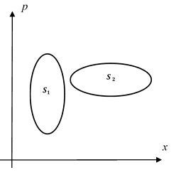
Phase Space

the two displayed areas being equal imply equal entropies.  When comparing different systems the action unit for entropy.  For more general systems we describe them in terms of probability distributions over the set of states, i.e. over phase space.  To then calculate the entropy we perform an area integral with

$$S = -k_B\int_{-\infty}^{\infty}\int_{-\infty}^{\infty} \rho\ln(\rho)dx dp$$

where  $\rho(x,p)$ is the probability density over phase space.

How Ambiguity Relates to Thermodynamic Entropy

Above two very different seeming definitions of entropy have been given.  One is a number associated with the evolution of thermodynamic systems and another is related to information, a quantifier of ambiguity.  To reconcile the two we need to understand how we describe and prescribe physical systems.

The state of a given classical physical system is completely determined by numerically specifying the configurations of all its components and then also their rates of change.  Then given a deterministic dynamic we can predict any past or future state (supposing no unaccounted for external influences perturbs the dynamics) exactly.  Even if there is some ambiguity, and hence entropy in our knowledge of the system state, that is to say, we at best know a probability distribution over the set of all possible states, we still, given deterministic dynamics, will not lose any information.  The informational entropy of the system will not change over time.  But no system is ever completely immune from unaccountable external influences.  For example, we have recently detected gravitational waves, the ripples of undulating space-time itself spreading outward from a distant cataclysmic merging of two black holes.  The very fact that our hypothesized physical systems exist in a larger universe means we can never completely remove random influences in the dynamics.    So a system evolving over time will of necessity increase in ambiguity unless and until that ambiguity, and hence entropy reaches some maximal value.

So we go back to one of the most basic thermodynamic thought experiments.  Two thermal systems at different temperatures are allowed to exchange energy with each other but with no net exchange of energy to the outside environment.  The environment can only “jostle the elbows” of the interactions, we make sure that it can draw from or add to the net energy.

So we have System 1, with all of its available energy maximally randomized so that its entropy is maximized to $S_1$ and it is at a given temperature $T_1$.  Likewise System 2, has it’s entropy maximized to $S_2$ and temperature is $T_2$.  When we consider the composite system which, classically will have a product state space that is the Cartesian product of the two-component systems we will see that their entropies will add to give the entropy of the composite system, $S=S_1 + S_2$.

Now we consider a small amount of dynamic evolution of the composite system wherein the total entropy must necessarily seek its maximal value.

$$\delta S = \delta S_1 + \delta S_2 = \frac{1}{T_1} \delta Q_1 + \frac{1}{T_2} \delta Q_2$$

But by our prescription any change in energy of one system will be balanced by an opposite change in the energy of the other, $\delta Q_2 = – \delta Q_1$.  We thus see that energy flowing in one direction (in a random fashion) will increase the entropy of the composite system.  Assume for the moment that $T_2 > T_1$.  Then we can, assuming the composite entropy increases derive the following:

$$\delta S > 0\quad \to\quad \left( \frac{1}{T_1} – \frac{1}{T_2}\right)\delta Q_1>0, \quad \to \quad \delta Q_1 > 0$$

since $$T_2>T_1 \to \frac{1}{T_1} > \frac{1}{T_2} \to \left(\frac{1}{T_1}-\frac{1}{T_2}\right)>0$$

So if energy is allowed to jump randomly between the two systems, energy flowing from the warmer to the cooler will allow the total entropy to increase.  This is a differential relationship momentarily treating the temperatures as constant.  But in point of fact, for most systems temperature increases with increasing energy and thus the cooler system will warm and the warmer system cool until both reach a common temperature and we can then describe that as the temperature of the composite system.  The entropy of the composite system has maximized and it has a definite temperature.

Maxwell’s Demon and Quantum Nature

There should still be something nagging at the mind of the astute reader here.  Take your physical system with its temperature and positive entropy and assume for a moment you can observe it completely.  You then remove any ambiguity in its state and instantly, without physically affecting the system you’ve reduced its entropy to zero.  Or less dramatically assume you measure one somewhat ambiguous property of that system, you will thereby have reduced it entropy by whatever amount that knowledge reduced its statistical ambiguity.  How can we change a system’s entropy without physically affecting it?

This issue, in another form, was best dramatized by James Clerk Maxwell’s infernal thought experiment.  Maxwell imagined two tanks of gas at equilibrium with a valve between them controlled by a demon who could observe the states of gas atoms near the valve.  The demon, when he saw a faster than average atom approaching from one side (and none from the other) would open the value just long enough to let the atom through.  Likewise, when a slower than average atom approached the valve from the other side he would open it just long enough to let that through.  This demon, using his knowledge of the states of the nearby particles could patiently, without changing the energies of any individual atoms or exerting any energy himself seemingly violate the 2nd Law of Thermodynamics.  The demon with pure knowledge is reversing the thermodynamically irreversible.  There are many variations bout the basic premise is this, knowledge can be utilized to affect changes of thermodynamic entropy.

There is a profound resolution to this seeming paradox.  There was an assumption that must be made in order to invoke Maxwell’s demon or any similar observation-based entropy change.  That assumption was stated above as “You can observe the physical system without affecting it.” In point of fact, acts of observation are changes in the physical state of the observer (or measuring device) caused by the specific state of the system.  The observer must causally interact with that which he observes and that interaction is always two-way.  What’s more, to amplify (and thereby copy arbitrarily) the information observed the measuring device must have a fundamentally thermodynamic component.

In short, to physically observe a system enough to decrease its entropy by a certain amount, the observing mechanism is required to increase entropy more elsewhere.  You see this with the heat sinks on amplifiers and the cryogenic systems for our more sensitive detectors.  Most importantly you see this as a fundamental aspect of the quantum description of nature.

Comments here