Struggles with the Continuum: Quantum Electrodynamics

 

 

Quantum field theory is the best method we have for describing particles and forces in a way that takes both quantum mechanics and special relativity into account. It makes many wonderfully accurate predictions. And yet, it has embroiled physics in some remarkable problems: struggles with infinities!

I want to sketch some of the key issues in the case of quantum electrodynamics, or ‘QED’. The history of QED has been nicely told here:

• Silvian Schweber, QED and the Men who Made it: Dyson, Feynman, Schwinger, and Tomonaga, Princeton U. Press, Princeton, 1994.

Instead of explaining the history, I will give a very simplified account of the current state of the subject. I hope that experts forgive me for cutting corners and trying to get across the basic ideas at the expense of many technical details. The nonexpert is encouraged to fill in the gaps with the help of some textbooks.

QED involves just one dimensionless parameter, the fine structure constant:

$$ \alpha = \frac{1}{4 \pi \epsilon_0} \frac{e^2}{\hbar c} \approx \frac{1}{137.036} . $$

Here $e$ is the electron charge, $\epsilon_0$ is the permittivity of the vacuum, $\hbar$ is Planck’s constant and $c$ is the speed of light. We can think of $\alpha^{1/2}$ as a dimensionless version of the electron charge. It says how strongly electrons and photons interact.

Nobody knows why the fine structure constant has the value it does! In computations, we are free to treat it as an adjustable parameter. If we set it to zero, quantum electrodynamics reduces to a free theory, where photons and electrons do not interact with each other. A standard strategy in QED is to take advantage of the fact that the fine structure constant is small and expand answers to physical questions as power series in $\alpha^{1/2}$. This is called ‘perturbation theory’, and it allows us to exploit our knowledge of free theories.

One of the main questions we try to answer in QED is this: if we start with some particles with specified energy-momenta in the distant past, what is the probability that they will turn into certain other particles with certain other energy-momenta in the distant future? As usual, we compute this probability by first computing a complex amplitude and then taking the square of its absolute value. The amplitude, in turn, is computed as a power series in $\alpha^{1/2}$.

The term of order $\alpha^{n/2}$ in this power series is a sum over Feynman diagrams with $n$ vertices. For example, suppose we are computing the amplitude for two electrons wth some specified energy-momenta to interact and become two electrons with some other energy-momenta. One Feynman diagram appearing in the answer is this:

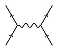
Here the electrons exchange a single photon. Since this diagram has two vertices, it contributes a term of order $\alpha$. The electrons could also exchange two photons:

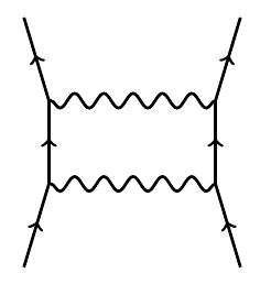
giving a term of $\alpha^2$. A more interesting term of order $\alpha^2$ is this:

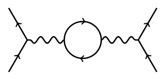
Here the electrons exchange a photon that splits into an electron-positron pair and then recombines. There are infinitely many diagrams with two electrons coming in and two going out. However, there are only finitely many with $n$ vertices. Each of these contributes a term proportional to $\alpha^{n/2}$ to the amplitude.

In general, the external edges of these diagrams correspond to the experimentally observed particles coming in and going out. The internal edges correspond to ‘virtual particles’: that is, particles that are not directly seen but appear in intermediate steps of a process.

Each of these diagrams is actually a notation for an integral! There are systematic rules for writing down the integral starting from the Feynman diagram. To do this, we first label each edge of the Feynman diagram with an energy-momentum, a variable $p \in \mathbb{R}^4$. The integrand, which we shall not describe here, is a function of all these energy-momenta. In carrying out the integral, the energy-momenta of the external edges are held fixed, since these correspond to the experimentally observed particles coming in and going out. We integrate over the energy-momenta of the internal edges, which correspond to virtual particles while requiring that energy-momentum is conserved at each vertex.

However, there is a problem: the integral typically diverges! Whenever a Feynman diagram contains a loop, the energy-momenta of the virtual particles in this loop can be arbitrarily large. Thus, we are integrating over an infinite region. In principle, the integral could still converge if the integrand goes to zero fast enough. However, we rarely have such luck.

What does this mean, physically? It means that if we allow virtual particles with arbitrarily large energy-momenta in intermediate steps of a process, there are ‘too many ways for this process to occur’, so the amplitude for this process diverges.

Ultimately, the continuum nature of spacetime is to blame. In quantum mechanics, particles with large momenta are the same as waves with short wavelengths. Allowing light with arbitrarily short wavelengths created the ultraviolet catastrophe in classical electromagnetism. Quantum electromagnetism averted that catastrophe — but the problem returns in a different form as soon as we study the interaction of photons and charged particles.

Luckily, there is a strategy for tackling this problem. The integrals for Feynman diagrams become well-defined if we impose a ‘cutoff’, integrating only over energy-momenta $p$ in some bounded region, say a ball of some large radius $\Lambda$. In quantum theory, a particle with a momentum of magnitude greater than $\Lambda$ is the same as a wave with a wavelength less than $\hbar/\Lambda$. Thus, imposing the cutoff amounts to ignoring waves of short wavelength — and for the same reason, ignoring waves of high frequency. We obtain well-defined answers to physical questions when we do this. Unfortunately, the answers depend on $\Lambda$, and if we let $\Lambda \to \infty$, they diverge.

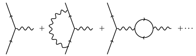
However, this is not the correct limiting procedure. Indeed, among the quantities that we can compute using Feynman diagrams are the charge and mass of the electron! Its charge can be computed using diagrams in which an electron emits or absorbs a photon:

Similarly, its mass can be computed using a sum over Feynman diagrams where one electron comes in and one goes out.

The interesting thing is this: to do these calculations, we must start by assuming some charge and mass for the electron — but the charge and mass we get out of these calculations do not equal the masses and charges we put in!

The reason is that virtual particles affect the observed charge and mass of a particle. Heuristically, at least, we should think of an electron as surrounded by a cloud of virtual particles. These contribute to its mass and ‘shield’ its electric field, reducing its observed charge. It takes some work to translate between this heuristic story and actual Feynman diagram calculations, but it can be done.

Thus, there are two different concepts of mass and charge for the electron. The numbers we put into the QED calculations are called the ‘bare’ charge and mass, $e_\mathrm{bare}$ and $m_\mathrm{bare}$. Poetically speaking, these are the charge and mass we would see if we could strip the electron of its virtual particle cloud and see it in its naked splendor. The numbers we get out of the QED calculations are called the ‘renormalized’ charge and mass, $e_\mathbb{ren}$ and $m_\mathbb{ren}$. These are computed by doing a sum over Feynman diagrams. So, they take virtual particles into account. These are the charge and mass of the electron clothed in its cloud of virtual particles. It is these quantities, not the bare quantities, that should agree with the experiment.

Thus, the correct limiting procedure in QED calculations is a bit subtle. For any value of $\Lambda$ and any choice of $e_\mathrm{bare}$ and $m_\mathrm{bare}$, we compute $e_\mathbb{ren}$ and $m_\mathbb{ren}$. The necessary integrals all converge, thanks to the cutoff. We choose $e_\mathrm{bare}$ and $m_\mathrm{bare}$ so that $e_\mathbb{ren}$ and $m_\mathbb{ren}$ agree with the experimentally observed charge and mass of the electron. The bare charge and mass chosen this way depend on $\Lambda$, so call them $e_\mathrm{bare}(\Lambda)$ and $m_\mathrm{bare}(\Lambda)$.

Next, suppose we want to compute the answer to some other physics problem using QED. We do the calculation with a cutoff $\Lambda$, using $e_\mathrm{bare}(\Lambda)$ and $m_\mathrm{bare}(\Lambda)$ as the bare charge and mass in our calculation. Then we take the limit $\Lambda \to \infty$.

In short, rather than simply fixing the bare charge and mass and letting $\Lambda \to \infty$, we cleverly adjust the bare charge and mass as we take this limit. This procedure is called ‘renormalization’, and it has a complex and fascinating history:

• Laurie M. Brown, ed., Renormalization: From Lorentz to Landau (and Beyond), Springer, Berlin, 2012.

There are many technically different ways to carry out renormalization, and our account so far neglects many important issues. Let us mention three of the simplest.

First, besides the classes of Feynman diagrams already mentioned, we must also consider those where one photon goes in and one photon goes out, such as this:

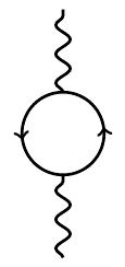
These affect the properties of the photon, such as its mass. Since we want the photon to be massless in QED, we have to adjust parameters as we take $\Lambda \to \infty$ to make sure we obtain this result. We must also consider Feynman diagrams where nothing comes in and nothing comes out — so-called ‘vacuum bubbles’ — and make these behave correctly as well.

Second, the procedure just described, where we impose a ‘cutoff’ and integrate over energy-momenta $p$ lying in a ball of radius $\Lambda$, is not invariant under Lorentz transformations. Indeed, any theory featuring the smallest time or smallest distance violates the principles of special relativity: thanks to time dilation and Lorentz contractions, different observers will disagree about times and distances. We could accept that Lorentz invariance is broken by the cutoff and hope that it is restored in the $\Lambda \to \infty$ limit, but physicists prefer to maintain symmetry at every step of the calculation. This requires some new ideas: for example, replacing Minkowski spacetime with 4-dimensional Euclidean space. In 4-dimensional Euclidean space, Lorentz transformations are replaced by rotations, and a ball of radius $\Lambda$ is a rotation-invariant concept. To do their Feynman integrals in Euclidean space, physicists often let time take imaginary values. They do their calculations in this context and then transfer the results back to Minkowski spacetime at the end. Luckily, there are theorems justifying this procedure.

Third, besides infinities that arise from waves with arbitrarily short wavelengths, there are infinities that arise from waves with arbitrarily long wavelengths. The former is called ‘ultraviolet divergences’. The latter is called ‘infrared divergences’, and they afflict theories with massless particles, like the photon. For example, in QED the collision of two electrons will emit an infinite number of photons with very long wavelengths and low energies, called ‘soft photons’. In practice, this is not so bad, since any experiment can only detect photons with energies above some nonzero value. However, infrared divergences are conceptually important. It seems that in QED any electron is inextricably accompanied by a cloud of soft photons. These are real, not virtual particles. This may have remarkable consequences.

Battling these and many other subtleties, many brilliant physicists and mathematicians have worked on QED. The good news is that this theory has been proved to be ‘perturbatively renormalizable’:

• J. S. Feldman, T. R. Hurd, L. Rosen and J. D. Wright, QED: A Proof of Renormalizability, Lecture Notes in Physics 312, Springer, Berlin, 1988.

• Günter Scharf, Finite Quantum Electrodynamics: The Causal Approach, Springer, Berlin, 1995

This means that we can indeed carry out the procedure roughly sketched above, obtaining answers to physical questions as power series in $\alpha^{1/2}$.

The bad news is we do not know if these power series converge. In fact, it is widely believed that they diverge! This puts us in a curious situation.

For example, consider the magnetic dipole moment of the electron. An electron, being a charged particle with spin, has a magnetic field. A classical computation says that its magnetic dipole moment is

$$ \vec{\mu} = -\frac{e}{2m_e} \vec{S} $$

where $\vec{S}$ is its spin angular momentum. Quantum effects correct this computation, giving

$$ \vec{\mu} = -g \frac{e}{2m_e} \vec{S} $$

for some constant $g$ called the gyromagnetic ratio, which can be computed using QED as a sum over Feynman diagrams with an electron exchanging a single photon with a massive charged particle:

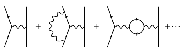
The answer is a power series in $\alpha^{1/2}$, but since all these diagrams have an even number of vertices, it only contains integral powers of $\alpha$. The lowest-order term gives simply $g = 2$. In 1948, Julian Schwinger computed the next term and found a small correction to this simple result:

$$ g = 2 + \frac{\alpha}{\pi} \approx 2.00232. $$

By now a team led by Toichiro Kinoshita has computed $g$ up to order $\alpha^5$. This requires computing over 13,000 integrals, one for each Feynman diagram of the above form with up to 10 vertices! The answer agrees very well with an experiment: in fact, if we also take other Standard Model effects into account we get agreement to roughly one part in $10^{12}$.

This is the most accurate prediction in all of science.

However, as mentioned, it is widely believed that this power series diverges! Next time I’ll explain why physicists think this, and what it means for a divergent series to give such a good answer when you add up the first few terms.