Addressing the “Classical Physics Is Wrong” Fallacy

One of the common questions or comments we get on PF is the claim that classical physics or classical mechanics (i.e. Newton’s laws, etc.) is wrong because it has been superseded by Special Relativity (SR) and General Relativity (GR), and/or Quantum Mechanics (QM). Such claims are typically made by either a student who barely learned anything about physics or by someone who has not had a formal education in physics. There is somehow a notion that SR, GR, and QM have shown that classical physics is wrong, and so, it shouldn’t be used.

There is a need to debunk that idea, and it needs to be done in the clearest possible manner. This is because the misunderstanding that results in such an erroneous conclusion is not just simply due to a lack of knowledge of physics, but rather due to something more inherent in the difference between science and our everyday world/practices. It is rooted in how people accept certain things and not being able to see how certain ideas can merge into something else under different circumstances.

Before we deal with specific examples, let’s get one FACT to straighten out:

Classical physics is used in an overwhelming majority of situations in our lives. Your houses, buildings, bridges, airplanes, and physical structures were built using classical laws. The heat engines, motors, etc. were designed based on classical thermodynamics laws. And your radio reception, antennae, TV transmitters, wi-fi signals, etc. are all based on the classical electromagnetic description.

These are all FACTS, not a matter of opinion. You are welcome to check for yourself and see how many of these were done using SR, GR, or QM. Most, if not all, of these, would endanger your life and the lives of your loved ones if they were not designed or described accurately. So how can one claim that classical physics is wrong, or incorrect, if they work, and work so well in such situations?

What is true is that we discovered a more accurate, and more general description of our world. In this description, it turns out that classical physics appears as a “simplification” or “approximation” whereby it becomes more and more valid as various parameters approach the common, everyday, terrestrial values. This is an extremely important point to remember because, since classical physics works under our ordinary situation, any new theory or description must somehow converge and look like the classical physics description under such ordinary conditions. Otherwise, this new theory must show that it produces the same set of results as classical physics for all of our known phenomena that classical physics can already accurately describe.

So in this part of the article, I will show two specific examples where the more general theory of SR and QM merge smoothly into the classical physics form when one adopts the appropriate approximation. This means that at some limit, both SR and QM descriptions will be the same as the classical description.

Example 1: Special Relativity Velocity Addition

The first example is from SR and deals with the velocity addition in different inertial reference frames. This is illustrated in the figure below:

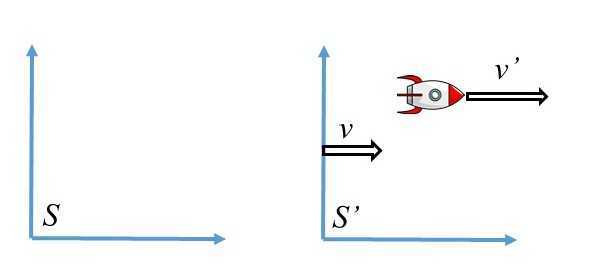
The reference frame S’ is moving with velocity v concerning reference frame S. A vessel is moving with velocity v’ concerning S’ frame. What is u, the velocity of that vessel concerning frame S?

The “normal” way to find this velocity is using what is known as Galilean transformation. Here, since both v and v’ and in the same direction, the velocity of the vessel concerning the S frame is a simple addition, i.e.

u = v + v’    (1)

Keep that result in mind.

Now let’s look at how we do this in SR, which is the more general description of such kinematics. Here, we use what is known as the Lorentz transformation. Using the figure from above as before, the velocity u of the vessel in the S frame is:

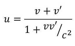    (2)

where c is the speed of light in a vacuum.

Now, this looks different than the Galilean transformation that we are used to in Eq. 1. This works for reference frame S’ at any velocity v, even if it approaches c. At that value, Eq. 1 does not work, and the velocity addition that we are used to fails miserably.

However, what happens when v«c, i.e. when reference frame S’ moves much slower than the speed of light? This is what we normally encounter, i.e. someone moving in a vehicle or an airplane. For v«c, Eq. 2 simplifies quite a bit. Without having to do any kind of Taylor series expansion on the denominator of Eq. 2, we can already see that the ratio vv’/c^2 « 1, i.e. it is a very small fraction less than one (v’ cannot be greater than c). This means that, to a good approximation, the denominator of Eq. 2 is essentially just 1.

When that happens, Eq. 2 then simplifies to u = v + v’, which is exactly Eq. 1! We got back our familiar result when we applied the more general equation (Eq. 2) to our normal, terrestrial condition! This means that all of the velocity addition equations and concepts that we already know using Galilean transformation are derivable from the more general Lorentz transformation equations. The Lorentz transformation is the more accurate, more encompassing description of velocity addition, while the Galilean transformation, which is what we know and are familiar with, is simply a special case for when the other reference frame is moving much slower than the speed of light. Eq. 1 isn’t wrong. It has a limited range of situations when it is valid or accurate enough.

Example 2: Quantum Mechanics Rate of Change of Momentum

In classical Newtonian mechanics, for an object with mass m, we know about Newton’s Second Law that relates the force F and the resulting acceleration a, which is

F = ma

This familiar equation can be written in a more general form, which is in terms of the time rate of change of momentum p, i.e.

F = dp/dt   (3)

We also know that force F can be related to the potential energy (V) gradient, i.e.

F = – dV/dx (in 1D)   (4)

So that is from the classical mechanics’ side. Let’s look at what it says on the QM side. Here, we use the Ehrenfest theorem, which says:

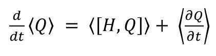   (5)

Here, H is the Hamiltonian, Q is an operator representing any observable, the square bracket represents the commutator, and the angled bracket represents the average value. These are all the standard notations used in QM.

So what if we want to find the time rate of change of the momentum, p? In QM, p is an operator representing the observable momentum. Thus, Eq. 5 becomes

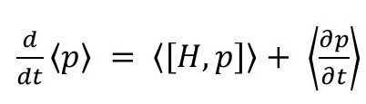   (6)

From here, it requires quite a bit of knowledge on how to perform the commutator and take the average. You may read the full derivation of it here. In the end, what you end up with is:

   (7)

This says that the time rate of change of the average value of the momentum p is equal to the average of the gradient of the potential energy V. But this equation is equivalent to Eq. 3 and 4 from classical mechanics! They have identical forms!

It says that what we typically measure in our everyday lives are the “average” values of many, many, many values at the QM level. The QM description has made the connection to the classical description under the condition that the QM observables have been averaged. Again, as in the case of velocity addition, we get back the classical description from a more general starting point, in this case, a QM description, upon applying a particular condition to the QM picture. It shows that the classical picture is not wrong. It is the average over a large number of QM observables.

Moral of the Story

1. Classical physics WORKS for our ordinary situation, so it HAS to be valid at some level.
2. Classical physics is derivable from SR and QM under special conditions that apply to our ordinary situation.
3. Any theory MUST have the ability to show that it merges with the classical description when applied to an ordinary situation.
4. This can only be shown mathematically. It cannot be shown convincingly via hand-waving or qualitative arguments. It is the equivalent mathematical form that shows that one theory can derive the other.

What this implies here is that, if there are more general and more accurate theories beyond QM, and SR/GR, then those theories must also show that they can be “simplified” into the mathematical forms of QM and SR/GR. Subsequent, more general theories must show that they can derive the mathematical forms of existing, already-working theories. The inability to do that will be a fatal flaw in any new theory.

I mentioned towards the beginning of this article that the inability to comprehend this concept of a more general idea merging and agreeing with something less general may have something to do with the differences between science and our everyday lives. It is unusual for many people to accept the possibility that a simplistic, less sophisticated, and different idea is a subset of a more general principle. The fact that one can actually start with a more general principle, apply certain criteria, and then get a seemingly different concept, is not something a lot of people are familiar with, or would even accept.

It is why for someone not trained in physics, the idea that classical mechanics can be derived from seemingly a different animal of QM or SR/GR would not even cross his/her mind. Yet, in science/physics, this is quite common. We always show how new ideas and theories will turn into the old, tested, and well-known ideas and theories under the appropriate parameters. It is very seldom that old theories are discarded wholesale.