Learn About the Friedmann Equation and the Cosmos

This is an introduction to cosmology for someone who has some knowledge of calculus and basic physics. In this tutorial, we will take a journey into the cosmos to study cornerstone ideas in cosmology and their derivations. Let’s begin our journey, by explaining the meaning of cosmology. Cosmology is the study of the origin, evolution, and eventual fate of the Universe. It comes from the Greek words –kosmos (world) and -logia (study of) ^[1].

Our exploration will start with the derivation of the Friedmann Equation. In the next chapters, we will try to understand the main elements that made our universe, the idea of dark matter and dark energy. After that we will go back in time to understand the origins of the Universe, we will study CMB (Cosmic Microwave Background), Baryogenesis, and Inflation.

Derivation of The Friedmann Equation

In this part of the journey, we will take a general look at the evolution and eventual fate of the Universe. The Friedmann Equation is the heart of these concepts. It explains the evolution of the Universe as a function of time for different types of models. Hence, it is important for us to derive and learn the Friedmann equation. However, before jumping to the Friedmann Equation, we should construct a basic understanding of cosmology. In the following two parts, we will try to understand the foundations of the Friedmann Equation.

The Cosmological Principle

In ancient times, our Greek ancestors looked up at the sky and wondered about our place in the universe. While observing the stars and planets, the Greeks developed a scientific approach to solving problems, leading to the creation of models of nature. The Greeks constructed conceptual models about the cosmos to explain what they observed in the sky ^[2].

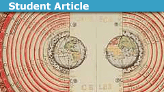
In their cosmic model, the Earth was in the center (Geocentric or Ptolemaic system), and other planets and stars were orbiting around the Earth.

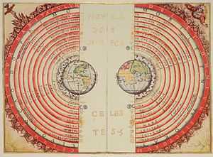
Fig. 1: Figure of the heavenly bodies, an illustration of the Ptolemaic geocentric system by Portuguese cosmographer and cartographer Bartolomeu Velho, 1568 (Bibliothèque Nationale, Paris) ^[3].

 

The Geocentric model was accepted until 1543 when Copernicus presented a new model, the Copernican Heliocentrism. It was a dramatic change in the history of science. Hence the reason it is called the Copernican revolution. It led to modern science. Copernican Heliocentrism positioned the Sun near the center of the universe, motionless with other planets orbiting around it. ^[4].

Copernicus proposed a principle that states that humans (the Earth or the Solar System) are not privileged observers of the universe ^[5]. This principle contains a vital idea about our place and how we look at the universe. In modern cosmology, this principle leads to the cosmological principle. The cosmological principle is a more robust version of the Copernicus Principle.

The cosmological principle states that wherever a person stands or looks, the universe should look the same. This description requires an idea of a homogeneous and isotropic universe or vice versa, since only in this case can cosmological principle make sense. Homogeneity states that the universe looks the same at each point, while isotropy states that the universe looks the same in all directions ^[6].

            Fig. 2: The Cosmological Principle ^[7]

 

The cosmological principle is fundamental to determining the geometry of the universe. For example, homogeneity and isotropy reduce the possible spaces that can exist due to symmetry. There exist only three types of homogeneous and isotropic spaces with simple topology: (a) flat space, (b) a three-dimensional sphere of constant positive curvature, and (c) a three-dimensional hyperbolic space of constant negative curvature ^[8]. Thus, the cosmological principle is the basis of the Friedmann Equation, which we will discuss later.
There is also something important to mention that the Universe is not strictly homogeneous and isotropic in small scales, less than $100 Mpc≈3.26×10^8ly$. It’s easy to observe such a result in this case. For example, no one thinks that sitting in a lecture theatre is the same as sitting in a bar. The interior of the Sun is a very different environment from the interstellar regions. Even on galactical scales, the Universe does not seem to look homogeneous and isotropic ^[6]. On the other hand, the cosmological principle becomes more important as we look at larger scales. About $100 Mpc$ or more ( while the radius of the Milky Way is about $15 pcs$ ), we can agree that the Universe is homogeneous and isotropic. Hence the cosmological principle is only valid within a range ^[9].

The Expanding Universe and Hubble’s Law

In 1929, Edwin Hubble discovered that the universe is expanding (before that in 1922 Alexander Friedmann put forward a set of equations that proposed that the universe might expand) ^[10]. Hubble observed that galaxies are moving away from us and surprisingly the further they are, the faster they move. Which we call, Hubble’s Law. However, before introducing Hubble’s Law in detail, we should first understand the idea of “expansion”.

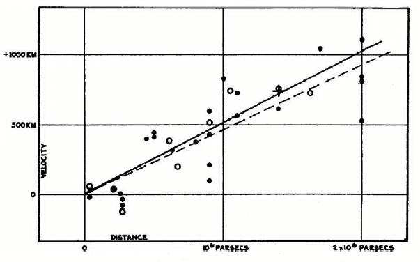
Fig. 3: Hubble’s graph of redshift versus distance ^[11].

 

“The expansion” of the universe (universe means space in this context) is called the metric expansion of space. A metric defines the concept of distance, by stating in mathematical terms how distances between two nearby points in space are measured, in terms of the coordinate system. Metric expansion is mathematically modeled by the FLRW metric which we will discuss in the next chapter.

The metric expansion of space is an intrinsic expansion whereby the scale of space itself changes. It means that the early universe did not expand “into” anything and does not require space to exist “outside” the universe. Instead, space itself changed, carrying the early universe with it as space grew. This is a completely different kind of expansion than the expansions of explosions seen in daily life. It also seems to be a property of the entire universe, rather than a phenomenon that applies just to one part of the universe or can be observed from “outside” it.

In cosmology, we cannot use a ruler to measure metric expansion, because our ruler will also be expanding (extremely slowly) ^[12]. In other words, we can’t use the cartesian coordinate system to express the expansion of the universe. Instead, try to picture a coordinate system with the grid lines expanding along with all of the objects in the Universe. So as time passes the grid system will expand or contract, as do the galaxies embedded on the grid lines. We call this a comoving coordinate system. Only in this special coordinate system observers (called comoving observers) will see the universe in an isotropic way, including the CMB radiation. Non-comoving observers will see regions of the sky systematically blue-shifted or red-shifted ^[13]. Meanwhile, we know that galaxies have some random motions (peculiar velocity) concerning the coordinate system. However, on large scales, due to homogeneity and isotropy, peculiar velocity will not be important ^[14].

Hubble’s Law

Now we can try to understand Hubble’s Law. Assume that the universe is homogeneous and isotropic. There are two galaxies, $A$ and $B$ embedded on the grid and suppose at $t$ galaxies have such position. The distance between the two galaxies will be;

 

 

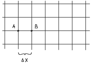
Fig. 4: A fictitious grid of coordinates following in unison the expanding, or contracting, Universe. The two galaxies shown remain at the same lattice point. Their grid distance remains the same, but their real distance may evolve with time ^[15].

 

$$D_{BA}=a(t)Δx~~~~~(2.1)$$

Here $a(t)$ is the scale factor, $Δx$ is the comoving distance and $D_{BA}$ is the proper distance. The comoving distance can be described as the unit distance between two galaxies. It can be set to any value at $t$  but once it’s set it doesn’t change with time. Comoving distance is a result of the coordinate system in which we embedded the galaxies on the grid. Hence the proper distance (actual distance) depends on the scale factor. Scale factor depends on the time which means the proper distance between two galaxies changes concerning time ^[14]. For example,  let us consider a simple case where $a(t)=t$ ,

$$D_{BA}=tΔx$$

Since $Δx$ is constant, we can say that;

$$D_{BA}∝t$$

the distance between galaxies will increase linearly as $t$ gets larger.

Now let’s calculate the velocity of  $B$ relative to $A$,

$$V_{BA}=\frac {dD} {dt}=\frac {d(a(t)Δx)} {dt}~~~~~(2.2)$$

Since $Δx$ doesn’t change with time;

$$V_{BA}=\dot a (t)Δx~~~~~(2.3)$$

We observe that $Δx$ can be canceled since it can be set to any value. Hence we can write;

$$\frac  {V_{BA}} {D_{BA}}=\frac  {\dot a (t)Δx} {a(t)Δx}=\frac  {\dot a (t)} {a(t)}~~~~~(2.4)$$

This ratio is what we call as Hubble parameter or expansion rate.

$$H=\frac  {\dot a (t)} {a(t)}~~~~~(2.5)$$

Now using $(2.4)$ and $(2.5)$ we can define the Hubble’s Law as;

$$V=HD~~~~~(2.6)$$

Where the unit of Hubble parameter is, $\left[ H\right]= \text{km}/\text{s}/\text{Mpc} ≡ 1/s$

The current Hubble parameter can be calculated as;

$$H({t_{\text{now}}}) \equiv H_0=\frac  {\dot a (t_0)} {a(t_0)}~~~~~(2.7)$$

Where,

$$H_0=67 \pm 0.46~\text{km}/\text{s}/\text{Mpc}$$

(Planck Mission-2015 results ^[17])

Some Misconceptions About The Hubble’s Law

Where is the center of the Universe? 

From Hubble’s Law, we can see that the velocity of the galaxies concerning us depends on the distance that we observed. This observation may lead us to think that, we are at the center of the universe since most of the galaxies appear to be moving away from us.

 

Fig. 5: An observer on galaxy B sees that every other galaxy is moving away, and the further they are, the faster they move (Hubble’s Law).

Fig. 6: An observer of galaxy A sees that every other galaxy is moving away, and the further they are, the faster they move (Hubble’s Law).

 

 

 

 

 

 

 

 

(Arrows represent the velocity of the galaxies according the Hubble’s Law, the magnitude of the arrows is proportional to galaxy velocities) ^[16]

 

But that’s not the real case. The observer of the galaxy $B$ and the galaxy $A$ will see the same thing from their perspective. Hence, we can’t talk about a real center because all observers will see that everything is moving away from them. It must be also true in the sense of the Copernicus Principle.

Is the universe expanding faster than the speed of light?

If we think more about Hubble’s Law, we can see that when we reach a certain distance it says that the object will reach the speed of light.

$$c=HD~~~~~(2.8)$$

Where $c$ is the speed of light. Hence, the distance will be;

$$D=\frac  {c} {H} ≅ \frac  {299792 km/s} {67~\text{km}/\text{s}/\text{Mpc}}≈4500Mpc$$

Because of this reason, galaxies further than $4500Mpc$  may seem to exceed the speed of light and there’s nothing wrong with it ( where the observable universe radius is $28500Mpc$ ). There are a couple of reasons behind it. In this model, since the galaxies are embedded on the grid, the distance between galaxies is not expanding due to their velocity but space itself which is expanding, and it drags the galaxies with it. We can see the galaxies that are further than that distance since the light that is reaching us is coming from the past where the object was still within the limit of this distance ^[18]. Furthermore, special relativity is not violated, because it refers to the relative speeds of objects passing each other, and cannot be used to compare the relative speeds of distant objects ^[19]. The reason for this is, that in large cosmic scales, space is curved but the theory is “special” in that, it only applies in the special case where the curvature of spacetime due to gravity is negligible ^[20].

The Friedmann Equation

In 1922, Alexander Friedmann proposed a set of equations that can describe the expansion of the universe ^[21]. He used general relativity to derive these equations but for simplicity, we will use the Newtonian approach and we will derive the same equation that Friedmann did.

The gravitational force between two massive objects can be described as;

$$F={\frac  {MmG} {r^2}}~~~~~(3.1)$$

Where $G$ is the gravitational constant, $r$ is the distance between two objects, $m$ and $M$ are the mass of the objects. Meantime the gravitational potential energy can be described as;

$$V=-{\frac  {MmG} {r}}~~~~~(3.2)$$

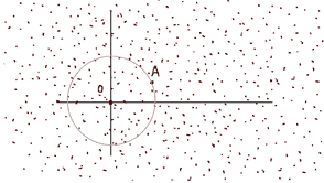
Fig. 7: The particle A at a radius only feels gravitational attraction from the shaded region. Any gravitational attraction from the material outside cancels out, according to Newton’s Theorem.

 

Consider a homogeneous and isotropic universe. There’s a particle $A$ (we can treat galaxies as particles in large scales and ignore their peculiar velocities) with a mass of $m$ and we want to find the force that acts on that particle due to other galaxies. Newton’s Shell theorem says, that in a frame of reference where everything is isotropic concerning the origin, it doesn’t even have to be homogeneous. If we want to know what the gravitational force exerted on a particle of mass $m$, then we can draw a sphere centered at the origin and go through the particle as shown in Fig.7. Assuming that all the particles in the sphere (where total mass is $M$ ) concentrated on the origin, $O$ and ignore all the mass in the universe farther away than $m$, from the origin because it’s the net force on $A$  is null. Then the force exerted on $A$ can be calculated as the force due to a unique point mass located at $O$ ^[22].

In this case, the total force on the particle can be calculated as;

$$F_{total}={\frac  {MmG} {r^2}}~~~~~(3.3)$$

Where $M$  is the total mass inside the sphere.

Let’s try to calculate the total energy of the particle $A$.

$$E_{total}=KE+PE~~~~~(3.4)$$

Where $KE$ is the kinetic energy and $PE$  is the gravitational potential energy of that particle.

The total energy of the particle can be useful to understand and calculate the motion. If the total energy of this particle is greater than zero it will escape, and it will never return. If it’s zero the speed of the object will just as asymptotically approach to zero but never will, and last when total energy is negative the particle will just fall to the center.

$$E_{total}=\frac {1} {2}mv^2-{\frac  {MmG} {r}}~~~~~(3.5)$$

Inserting $(2.3)$ on $(3.5)$ we get,

$$E_{total}=\frac {1} {2}m(\dot a (t)Δx)^2-{\frac  {MmG} {r}}~~~~~(3.6)$$

Since in this case, $r=a(t)Δx$

We can divide both sides of the equation to $m$  and multiply by $2$.

$$\frac {2E} {m}=(\dot a (t)Δx)^2-\frac {2MG} {a(t)Δx}~~~~~(3.7)$$

Instead of $M$ we can use the density of the particles inside the sphere,

$$M=\rho \frac {4} {3}\pi (a(t)Δx)^3~~~~~(3.8)$$

Dividing $(3.7)$ to $(Δx)^2$  and inserting $(3.8)$, we get;

$$\frac {2E} {ma^2(t)}=\frac {\dot a^2 (t)} {a^2(t)}-\frac {8\pi \rho G} {3}~~~~~(3.9)$$

Where, $-2E/m=k$. This transition can be thought of as changing the equation to relativity, from Newtonian mechanics and $k$ can be expressed as a curvature of space.

There are three possible values that $E$  can take: positive, negative, or zero.

1. If $E<0$  then, $k>0$  (we will see that, it’s exactly $1$) and represents a three-dimensional sphere of constant positive curvature.
2.  If $E=0$ then, $k=0$  and represents a flat space.
3. If $E>0$ then, $k<0$  (we will see that, it’s exactly $-1$) and represents a three-dimensional hyperbolic space of constant negative curvature ^[23].

 

Fig. 8: Space-time histories for Friedmann’s cosmological models in which the spatial curvature of the universe is positive, zero, and negative (left to right) ^[24].

 

Now we can arrange the $(3.9)$ respect to $k$  and we get;

$$\frac {\dot a^2 (t)} {a^2(t)}=\frac {8\pi \rho G} {3}-\frac {k} {a^2(t)}~~~~~(3.10)$$

From $(2.5)$ we can rewrite as;

$$H^2=\frac {8\pi \rho G} {3}-\frac {k} {a^2(t)}~~~~~(3.11)$$

This is the Friedmann Equation without the cosmological constant.

Although Newtonian cosmology can reproduce the chief results derived from Einstein’s equations, it is essentially incomplete, for several reasons. We need general relativity to justify the neglect of all matter outside a sphere of radius $r$ in calculating the gravitational potential energy. We cannot use Newtonian mechanics when the medium itself consists of particles with relativistic local velocities ^[26]. Also in such large scales, curvature of space becomes more important which means we can’t use Newtonian mechanics as a fully correct approach.

In the next chapter, we will further investigate the Friedmann Equation. We will explore the FLRW metric and the fluid equation and we will solve the Friedmann equation for some models.

Next Chapter: A Journey Into the Cosmos – FLRW Metric and The Friedmann Equation

References

1-Cosmology (https://en.wikipedia.org/wiki/Cosmology). (para. 1).

2-Bennett, Donahue, Schneider and Voit (2012). The essential cosmic perspective (6th ed.). (p. 62).

3-Geocentric Model (https://en.wikipedia.org/wiki/Geocentric_model). (para.1).

4- Bennett, Donahue, Schneider and Voit (2012). The essential cosmic perspective (6th ed.). (p. 65).

5-Copernican Principle (https://en.wikipedia.org/wiki/Copernican_principle). (para. 1).

6-Riddle, A. (2003). An introduction to modern cosmology (p. 2).

7-The Cosmological Principle (http://abyss.uoregon.edu/~js/cosmo/lectures/lec05.html)

8- Mukhanov, V. (2005). Physical foundations of cosmology (p. 14).

9- Mukhanov, V. (2005). Physical foundations of cosmology (p. 3).

10-Hubble’s Law (https://en.wikipedia.org/wiki/Hubble%27s_law). (para. 2)

11-Hubble’s graph of redshift (https://cosmictimes.gsfc.nasa.gov/online_edition/1929Cosmic/expanding.html)

12- Metric expansion of space (https://en.wikipedia.org/wiki/Metric_expansion_of_space).

13-Comoving and proper distances (https://en.wikipedia.org/wiki/Comoving_and_proper_distances#Comoving_coordinates) (para. 3)

14-Jaffe, A. (2012). Cosmology lecture notes (p. 3) (http://astro.imperial.ac.uk/sites/default/files/cosmology.pdf)

15-Susskind, L. (2013). Cosmology lecture notes (p. 10) (https://www.lapasserelle.com/cosmology/lesson_1.pdf )

16-Where’s the center of the big bang? (http://www.astro.ucla.edu/~wright/nocenter.html)

17-Planck Collaboration. (2015). Planck 2015 results. XIII. Cosmological parameters (p.6) (https://arxiv.org/abs/1502.015899)

18-Rothstein, D. (2016, February 10). Is the universe expanding faster of the speed of light? Retrieved from (http://curious.astro.cornell.edu/about-us/104-the-universe/cosmology-and-the-big-bang/expansion-of-the-universe/616-is-the-universe-expanding-faster-than-the-speed-of-light-intermediate)

19- Riddle, A. (2003). An introduction to modern cosmology (p. 21).

20-Special Relativity (https://en.wikipedia.org/wiki/Special_relativity ). (para. 6).

21-Friedmann Equations (https://en.wikipedia.org/wiki/Friedmann_equations#cite_note-af1922-1). (para. 1).

22- Susskind, L. (2013). Cosmology lecture notes (p. 17) (https://www.lapasserelle.com/cosmology/lesson_1.pdf )

23- Susskind, L. (2013). Cosmology lecture notes (p. 30) (https://www.lapasserelle.com/cosmology/lesson_1.pdf )

24-Space-Time Histories for Friedmann Equation (https://www.climate-policy-watcher.org/coarse-graining/our-expanding-universe.html)

25-Weinberg, S. (1972). Gravitation and cosmology: principles and applications of the general theory of relativity (p. 475).