Lesson on Entanglement Entropy in Quantum Field Theory

1. Part 1: Quantum Mechanics

[This article expects the reader to have some experience with quantum field theory and path integrals]

[I should also make a disclaimer here, some parts of this article use some results from conformal field theory which is beyond my knowledge. So I have to just state the results in those parts. I’d appreciate comments from more knowledgeable people.]

In this part, I’m going to take a look at the notion of Entanglement Entropy(EE), for a Quantum Field Theory(QFT). It’s obvious that things are going to be different. In QM we always could recognize if we’re looking at a composite system or not and we always could recognize the subsystem of a composite system simply because we were dealing with discrete kinds of things. But fields encompass some notion of continuity and so there is no default and unique way of decomposing them into subsystems. We should also consider that a QFT is defined on spacetime and we should be able to deal with that too, although in a trivial manner.

So now we should define at least two subsystems that are complementary and together make up the whole field. What we do first, is to consider a constant time slice of the background spacetime and then simply call it space*. Now we can consider a region of the space and think about the entanglement of this part of the field with the rest of the field. But before we continue, I should point out that a field theory has an infinite number of modes and each of these modes is involved in the entanglement of the two regions. So we expect the result to be divergent. We also know that we’re dealing with a local theory, so each point can only directly affect its neighbors and this means that any connection a region has with its outside, has to be through its boundary. So we expect the result to be proportional to the area of the boundary of the region.

So, let’s start to calculate the entanglement entropy of a region of a quantum scalar field in its ground state with the rest of the field. But for that, we need to be able to write down the state of the field theory in a way that enables us to do the required calculations. It turns out that this can be done using path integrals.

 

The state of a quantum field

An introductory course on quantum field theory usually focuses on the canonical quantization of a classical field theory and the emergence of particles from that and then uses the multi-particle Fock states of these emergent particles. But in this subject, these emergent particles don’t interest us. Actually, we’re going to do all the calculations for the vacuum state which has no particle. We need to use a formalism that enables us to recognize different regions of the field and lets us do all those tracing-out stuff that we did with the good old QM. So the formalism that we’re going to use, is the functional approach to QFT along with some knowledge about path integrals.

In the functional approach, we follow a parallel path with QM. We associate a state to the whole quantum field which is the probability amplitude for the field to be in one particular configuration. This state solves a functional differential equation which is actually a functional Schrodinger equation with the proper functional Hamiltonian. So we now can use a lot of mathematical tricks from QM. One of these tricks that we are going to use now, is writing the ground state of the system using a path integral.

At first we should consider that $\displaystyle \langle\phi,t=0|\psi,t\rangle=\langle \phi|\psi,t\rangle\propto \int_{\xi(t=0,x)=\phi(x)}^{\xi(t,x)=\psi(x)}D\xi e^{-iS[\xi]}$. Now if the Hamiltonian of the system is time-independent, we’ll have($\{\eta_b\}$ are the energy eigenstates):

 

$\displaystyle \langle \phi|\psi,t\rangle=\langle \phi|e^{iHt}|\psi\rangle=\sum_b \langle\phi|e^{iHt}|\eta_b\rangle\langle\eta_b|\psi\rangle=\sum_b e^{iE_bt}\langle \phi|\eta_b\rangle\langle \eta_b|\psi\rangle=\sum_be^{iE_bt}\eta_b[\phi]\bar{\eta}_b[\psi]$

 

Now if we do a Wick rotation($t=-i\tau$), we’ll have $\langle \phi|\psi,\tau\rangle=\sum_be^{E_b\tau}\eta_b[\phi]\bar{\eta}_b[\psi]$. In first order, the $\tau\to -\infty$ limit of this expression is equal to zero and the first non-zero term comes from the ground state. We should now set $\psi=0$ because now $\psi$ is the boundary condition at infinity. So we have $\eta_0[\phi]\propto\langle \phi|0,\tau\to -\infty\rangle$. Now if we just change the name of $\eta_0[\phi]$ to $\Psi[\phi]$, we’ll find the formula $\displaystyle \Psi[\phi]\propto \int_{\xi(-\infty,x)=0}^{\xi(0,x)=\phi(x)} D\xi e^{-S[\xi]}$ for the ground state of a scalar field with a time-independent Hamiltonian(We should also do a separate Wick rotation in the exponential). A similar calculation gives $\displaystyle\bar \Psi [\psi]\propto \int_{\zeta(0,x)=\psi(x)}^{\zeta(\infty,x)=0}D\zeta e^{-S[\zeta]}$. Now we can write the density matrix of the system $\displaystyle \rho_{\phi\psi}\propto \int_{\xi(-\infty,x)=0}^{\xi(0,x)=\phi(x)}\int_{\zeta(0,x)=\psi(x)}^{\zeta(\infty,x)=0} D\xi D\zeta e^{-S[\xi]} e^{-S[\zeta]}$. It should be noted that $\phi$ and $\psi$ are actually acting as the indices of the density matrix. But because there are an infinite number of field configurations, we’re dealing with an $\infty \times \infty$ matrix.

If we wanted a total trace, we would set $\phi=\psi$ and integrate over the whole configuration space. So we would have $\displaystyle \rho \propto \int D\phi \int_{\xi(-\infty,x)=0}^{\xi(0,x)=\phi(x)}\int_{\zeta(0,x)=\phi(x)}^{\zeta(\infty,x)=0} D\xi D\zeta e^{-S[\xi]} e^{-S[\zeta]}$. If you really think about the meaning of a path integral, you would notice that what we’re actually doing here, is calculating the probability amplitude of going from 0 at $\tau\to-\infty$ to $\phi$ at $\tau=0$ and multiplying it by the probability amplitude of going from $\phi$ at $\tau=0$ to 0 at $\tau\to\infty$, which is equal to the 0-to-0 amplitude with the condition that the field is in the configuration $\phi$ at $\tau=0$. So when we integrate over all configuration space, we’re actually calculating the 0-to-0 amplitude itself which is equal to $\displaystyle\rho \propto \int_{\phi(-\infty,x)=0}^{\phi(\infty,x)=0} D\phi e^{-S[\phi]}$.

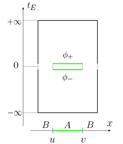
But we don’t want a full trace. For now, we need to trace out the parts of the field that lie outside of the region under consideration. So the beast that we need should have no free indices for points outside of the region, and two free different indices for points inside the region. We also know that those free indices are associated with $\tau=0$, but because we need two distinct conditions, we will tear up the $\tau=0 \ , \ x\in Region$ line to $\tau=0^{\pm}$. This seems to be a formidable beast. But maybe we can somehow turn our full trace formula into it. This idea comes from the realization that the beast we want is actually a regular full trace for points outside of the region and a regular density matrix for points inside. So we just need to interfere in the integral and make it give us something that depends on two arbitrary fields for points inside the region. But this seems to be a perfect job for a bunch of delta functions. This line of thinking gives us the following formula for the reduced density matrix:

$\displaystyle [\rho_{_{reduced}}]_{\phi_+\phi_-}\propto \int D \phi e^{-S[\phi]} \prod_{x\in Region}\delta\left( \phi(0^+,x)-\phi_+(x) \right)\delta\left( \phi(0^-,x)-\phi_-(x) \right)$

 

 

What to do with $Tr(\rho \ln \rho)$?

In the case of QM, calculating $Tr(\rho \ln \rho)$ was not much of a challenge. But if you take a look at the above formula, you realize that its not that simple this time. So maybe we can find a simpler way, one that doesn’t involve any logarithms. Fortunately such a way exists. We just need to consider the formula $\displaystyle S=-\lim_{n\to 1}\frac{\partial}{\partial n}\ln Tr(\rho^n)$. Let’s see how this formula reduces to what we want:

 

$\displaystyle \lim_{n\to 1}\frac{\partial}{\partial n}\ln Tr(\rho^n)=\lim_{n\to 1}\frac{\frac{\partial}{\partial n}Tr(\rho^n)}{Tr(\rho^n)}=\lim_{n\to 1}\frac{\frac{\partial}{\partial n}\sum_b \rho_b^n}{\underbrace{Tr(\rho^n)}_{ \to 1 \ as \ n\to 1}}=\lim_{n\to 1}\sum_b \rho_b^n \ln \rho_b=Tr(\rho \ln \rho)$

 

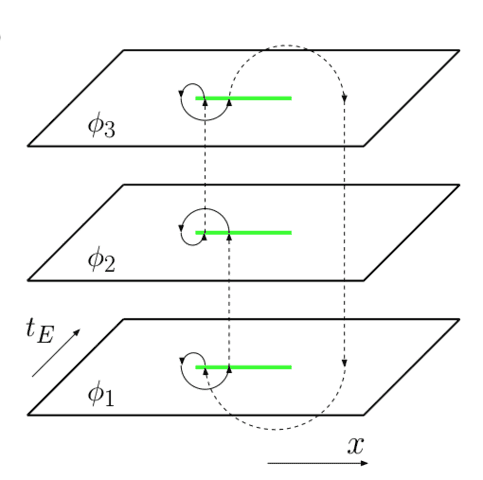
So now we need to calculate the nth power of the reduced density matrix. As I said before, the role of the indices of the matrix is played by the two free fields in the formula for the density matrix. So the multiplication of matrices is done by putting n reduced density matrices together and equating the fields between them and then integrating over those fields. After that, we should take the trace of the result which means equating the remaining fields and integrating over them. So eventually we want to equate all the fields and integrate over them. But it should be noted that this is not a typical path integral calculation. What we are doing is actually sewing together n complex planes together which gives an n-sheeted Riemann surface over which the reduced density matrix is integrated.

 

What to do with this mess?

Obviously, we got ourselves into serious trouble with this calculation. What should we do now? Well, there is actually a way to get rid of the Riemann surface and instead integrate over n disconnected sheets. But we should put some interesting boundary conditions over the fields(Where u and v represent the two end-points of the interval under consideration):

 

$\phi_k(e^{2\pi i}(x-u))=\phi_{k+1}(x-u) \ , \ \phi_k(e^{2\pi i}(x-v))=\phi_{k-1}(x-v)$

 

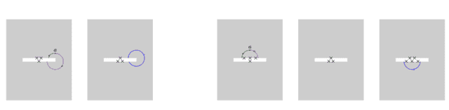
But how can we enforce these boundary conditions? We just put a bunch of operators in the theory whose job is to twist each field in the proper point and then connect it to the next or previous field in the next or previous sheet. These are called twist operators, for obvious reasons. These operators are defined as below:

 

$T_n \equiv T_\sigma \ \ , \ \ \ \ \ \sigma \ \ \ : i\to i+1 \mod n$

$\tilde T_n \equiv T_{\sigma^{-1}} \ \ , \ \ \ \ \ \sigma^{-1} \ \ \ : i+1\to i \mod n$

 

So now we just need to calculate the quantity $\prod_k\langle T_n^{(k)}\tilde T_n^{(k)}\rangle$. But it still seems to be something we can’t calculate.  But if the field theory we’re dealing with is a conformal field theory, these twist operators are primary operators which means we already know their two-point function.  So knowledge from conformal field theory gives us the result of this calculation as $S=\frac c 3 \ln \frac l a$, where $l=u-v$, a is the UV cut-off of the theory and c is the central charge of the conformal field theory.

One interesting thing to notice is that this result is not extensive, which is what we usually expect from entropy. I should also mention that a simple transformation can be used to make this same calculation give us the entanglement entropy in a conformal field theory at finite temperature. The result is $S=\frac c 3 \ln \left( \frac \beta a \sinh \left( \frac {\pi l} \beta \right) \right)$. The high-temperature limit of this formula is $\frac {\pi c}3 lT$ which is extensive, as we expect from thermal entropies.

* I think this means that now we are limited to globally hyperbolic spacetimes, but I’m not sure. Maybe there is some workaround that lets us use more general spacetimes. Let me know if you’re more familiar with this.